数据准备
这里使用的是公开的Expedia个性化酒店搜索中的部分数据。数据介绍:
| 列名 | 数据类型 | 描述 |
| srch_id | Integer | 搜索ID |
| date_time | Date/time | 搜索时间 |
| site_id | Integer | Expedia不同的站点(例如:Expedia.com, Expedia.co.uk, Expedia.co.jp,..) |
| visitor_location_country_id | Integer | 浏览者所在国家 |
| visitor_hist_starrating | Float | 用户历史预订的平均星级,null代表没有历史记录 |
| visitor_hist_adr_usd | Float | 用户历史预订的平均房价,null代表没有历史记录 |
| prop_country_id | Integer | 酒店所在的国家 |
| prop_id | Integer | 酒店ID |
| prop_starrating | Integer | 酒店星级(1-5),0代表酒店没有星级 |
| prop_review_score | Float | 酒店点评分(0-5之间),0.5为梯度。0代表没有点评 |
| prop_brand_bool | Integer | 1为品牌联锁,0为个体酒店 |
| prop_location_score1 | Float | 酒店所在位置的得分 |
| prop_location_score2 | Float | 酒店所在位置的得分 |
| prop_log_historical_price | Float | 酒店上次交易时的价格,如果为0,则代表近期没有交易 |
| position | Integer | 酒店在搜索结果中的位置 |
| price_usd | Float | 外显价格,不同国家显示的不同(有些包含税费有些不包含) |
| promotion_flag | Integer | 如果有特价促销,显示为1,否则显示0 |
| gross_booking_usd | Float | 每次交易的利润 |
| srch_destination_id | Integer | 酒店搜索的目的地ID |
| srch_length_of_stay | Integer | 搜索的入住天数 |
| srch_booking_window | Integer | 搜索的提前天数 |
| srch_adults_count | Integer | 搜索成人数量 |
| srch_children_count | Integer | 搜索儿童数量 |
| srch_room_count | Integer | 搜索房间数 |
| srch_saturday_night_bool | Boolean | 搜索的入住日期是否包含周六 |
| srch_query_affinity_score | Float | 酒店平均点击率,0代表没有点击或没有展示 |
| orig_destination_distance | Float | 用户搜索时位置和酒店位置之间的距离,如果为NULL则表示距离无法被计算 |
| random_bool | Boolean | 1表示返回的结果是随机的,0表示正常的结果返回 |
| comp1_rate | Integer | 1代表Expedia比竞争对手的价格低,0表示和竞争对手的价格一样。-1表示Expedia的价格比竞争对手高。NULL代表数据缺失。 |
| comp1_inv | Integer | 如果竞争对手此酒店不可定,则返回1,如果都可定,则返回0。NULL代表没有竞品数据 |
| comp1_rate_percent_diff | Float | 与竞对价格差的百分比,NULL代表没有数据 |
| comp2_rate | Integer | 同上 |
| comp2_inv | Integer | 同上 |
| comp2_rate_percent_diff | Float | 同上 |
| comp3_rate | Integer | 同上 |
| comp3_inv | Integer | 同上 |
| comp3_rate_percent_diff | Float | 同上 |
| comp4_rate | Integer | 同上 |
| comp4_inv | Integer | 同上 |
| comp4_rate_percent_diff | Float | 同上 |
| comp5_rate | Integer | 同上 |
| comp5_inv | Integer | 同上 |
| comp5_rate_percent_diff | Float | 同上 |
| comp6_rate | Integer | 同上 |
| comp6_inv | Integer | 同上 |
| comp6_rate_percent_diff | Float | 同上 |
| comp7_rate | Integer | 同上 |
| comp7_inv | Integer | 同上 |
| comp7_rate_percent_diff | Float | 同上 |
| comp8_rate | Integer | 同上 |
| comp8_inv | Integer | 同上 |
| comp8_rate_percent_diff | Float | 同上 |


使用的数据:
- 选择数据点最多的酒店prop_id=104517
- 选择visitor_location_country_id=219(219代表美国)来统一price_usd列
- 选择search_room_count=1
- 选择我们需要的其他特征:date_time、price_usd、srch_booking_window和srch_saturday_night_bool
import pandas as pd
import matplotlib.pyplot as plt
train = pd.read_csv('data/train.csv')
df = train.loc[train['prop_id'] == 104517]
df = df.loc[df['visitor_location_country_id'] == 219]
df = df.loc[df['srch_room_count'] == 1]
df = df[['date_time', 'price_usd', 'srch_booking_window', 'srch_saturday_night_bool']]
df = df.loc[df['price_usd'] < 5584] #去除特别异常的数据
df['date_time'] = pd.to_datetime(df['date_time'])
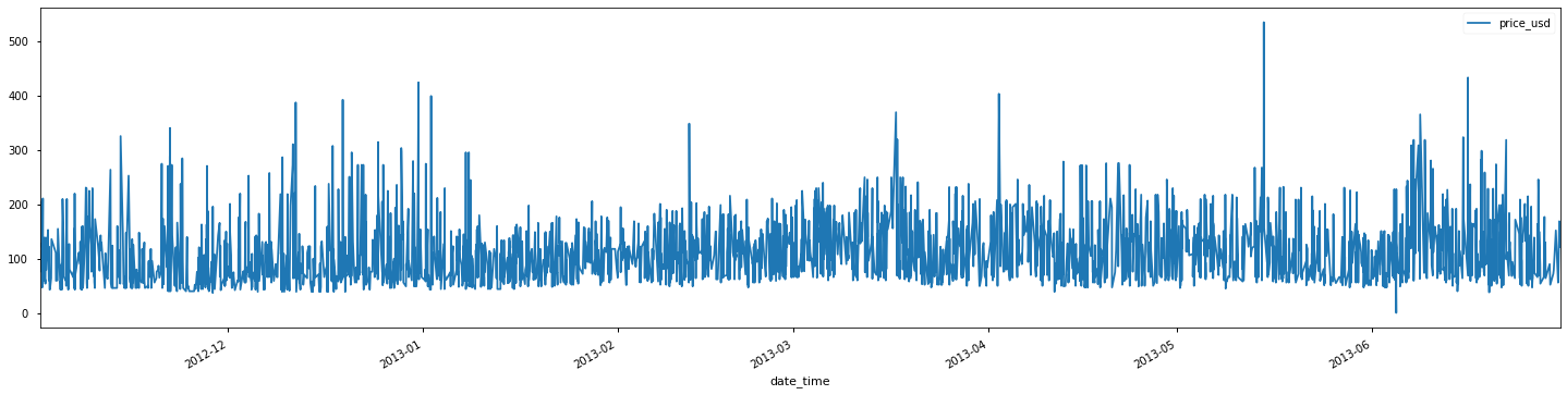
df.plot(x='date_time', y='price_usd', figsize=(20,5))
plt.show()
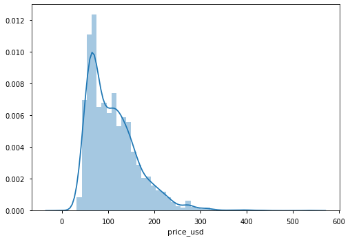
数据观察
整体价格分布:
import seaborn as sns
sns.distplot(df['price_usd'])
查看包含周六与不包含周六的价格分布:
a = df.loc[df['srch_saturday_night_bool'] == 0, 'price_usd']
b = df.loc[df['srch_saturday_night_bool'] == 1, 'price_usd']

plt.figure(figsize=(10, 6))
plt.hist(a, bins=50, alpha=0.5, label='Search Non-Sat Night')
plt.hist(b, bins=50, alpha=0.5, label='Search Sat Night')
plt.legend(loc='upper right')
plt.xlabel('Price')
plt.ylabel('Count')
plt.show()

包含周六的价格明显偏高。说明价格与是否包含周六强相关。
再来看看其他的字段:
sns.pairplot(df)
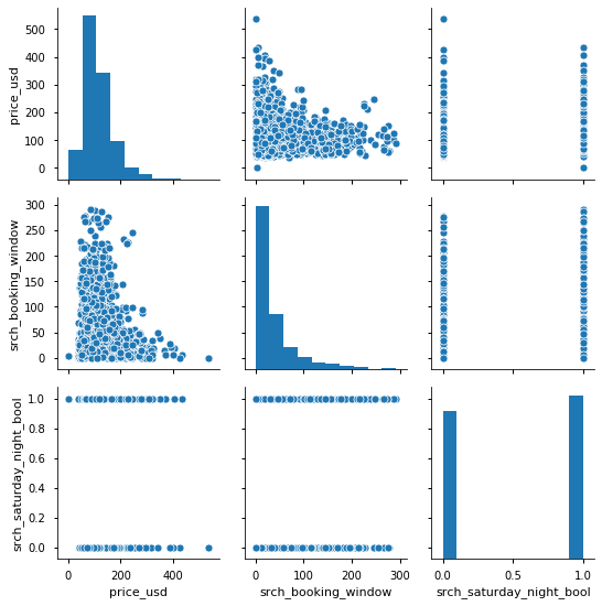
Booking Window与价格的关系:
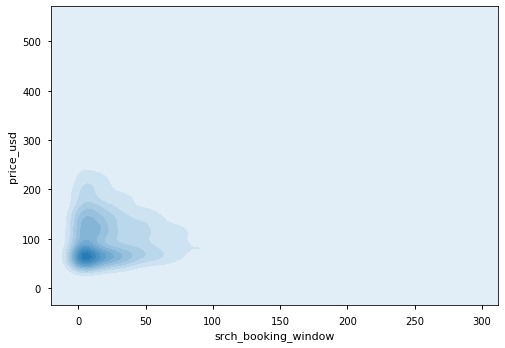
发现还是存在一定的相关性。
基于聚类的异常检测
from sklearn.cluster import KMeans

train_data = df[['price_usd', 'srch_booking_window', 'srch_saturday_night_bool']]
n_cluster = range(1, 20)
kmeans = [KMeans(n_clusters=i).fit(train_data) for i in n_cluster]
scores = [kmeans[i].score(train_data) for i in range(len(kmeans))]

fig, ax = plt.subplots(figsize=(10, 6))
ax.plot(n_cluster, scores)
plt.xlabel('Number Of Clusters')
plt.ylabel('Score')
plt.title('Elbow Curve')
plt.show()
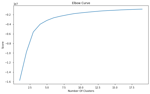
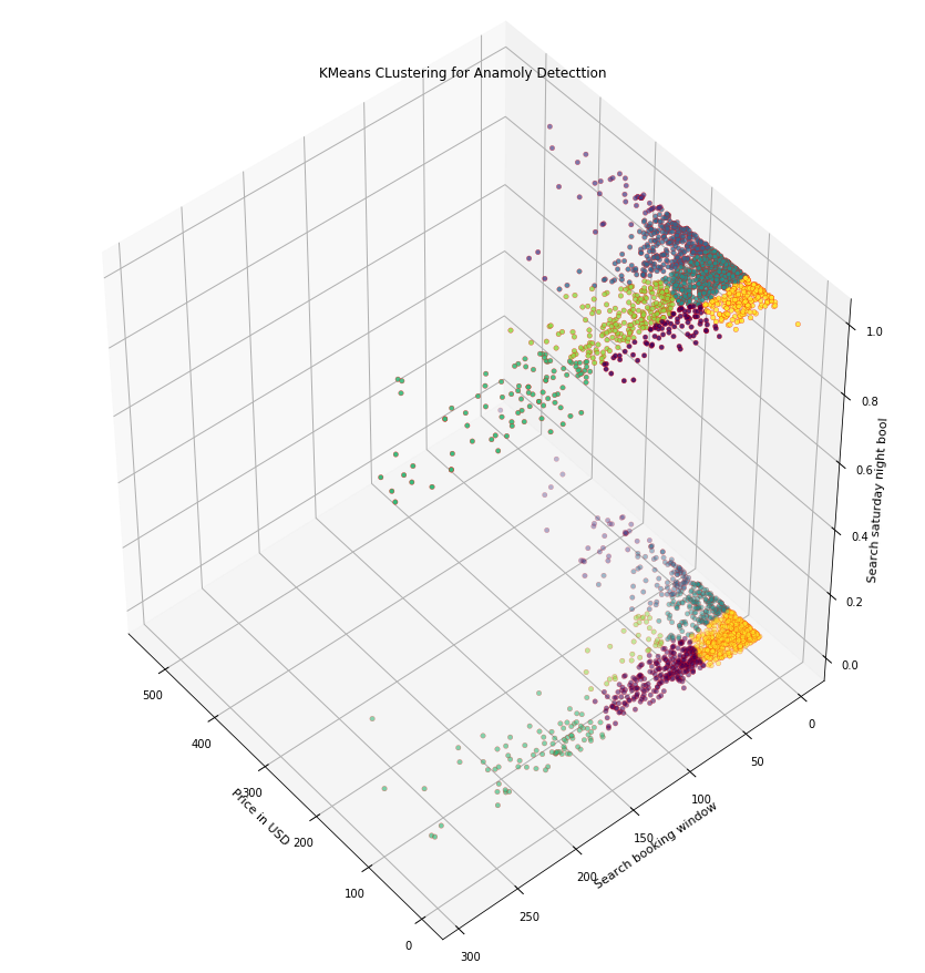
从上图,我们选定k=7。然后绘制3D的簇:
X = train_data.reset_index(drop=True)
km = KMeans(n_clusters=7)
km.fit(X)
km.predict(X)

import numpy as np
from mpl_toolkits.mplot3d import Axes3D

fig = plt.figure(1, figsize=(12, 12))
ax = Axes3D(fig, rect=[0, 0, 0.95, 1], elev=45, azim=140)
labels = km.labels_
ax.scatter(X.iloc[:, 0], X.iloc[:, 1], X.iloc[:, 2], c=labels.astype(np.float), edgecolor='r')
ax.set_xlabel('Price in USD')
ax.set_ylabel('Search booking window')
ax.set_zlabel('Search saturday night bool')
plt.title('KMeans CLustering for Anamoly Detecttion')
plt.show()
前只是进行了聚类,如何确定聚类中的哪些点是异常点呢?先来看看各个特征的重要性:
from sklearn.preprocessing import StandardScaler

data = df[['price_usd', 'srch_booking_window', 'srch_saturday_night_bool']]
X = data.values
X_std = StandardScaler().fit_transform(X)

# Calc eigenveccor & eig_vals of covar matrix
mean_vec = np.mean(X_std, axis=0)
cov_mat = np.cov(X_std.T)
eig_vals, eig_vecs = np.linalg.eig(cov_mat)

# eig_val, eig_vecs tuple
eig_pairs = [(np.abs(eig_vals[i]), eig_vecs[:, i]) for i in range(len(eig_vals))]
eig_pairs.sort(key=lambda x: x[0], reverse=True)

# Calc explained var from eig_vals
total = sum(eig_vals)

# Individual explained var
var_exp = [(i / total) * 100 for i in sorted(eig_vals, reverse=True)]

# Cumulative explained var
cum_var_exp = np.cumsum(var_exp)

plt.figure(figsize=(8, 8))
plt.bar(range(len(var_exp)), var_exp,
alpha=0.5, align='center',
label='individual explained var',
color='r'
)

plt.step(range(len(cum_var_exp)), cum_var_exp,
where='mid',
label='cumulative explained var')

plt.xlabel('principal components')
plt.ylabel('explained var ratio')
plt.legend(loc='best')
plt.show()
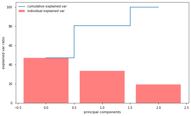
我们可以看到,第一个成分解释了解释了几乎50%的方差,第二个成分解释了超过30%的方差。没有哪一个成分是可以忽略不计的。前两个成分包含了超过80%的信息,这里是用主成分分析PCA降维到二维后再进行聚类:
from sklearn.decomposition import PCA

# Take useful feature and standardize them
data = df[['price_usd', 'srch_booking_window', 'srch_saturday_night_bool']]

# Standardize features
X_std = StandardScaler().fit_transform(X)
data = pd.DataFrame(X_std)

# Reduce components to 2
pca = PCA(n_components=2)
data = pca.fit_transform(data)

# Standardize 2 new features
scaler = StandardScaler()
np_scaled = scaler.fit_transform(data)
data = pd.DataFrame(np_scaled)

kmeans = [KMeans(n_clusters=i).fit(data) for i in n_cluster]
df['cluster'] = kmeans[7].predict(data)
df.index = data.index
df['principal_feature1'] = data[0]
df['principal_feature2'] = data[1]
df['cluster'].value_counts()

# plot the different clusters with the 2 main features
fig, ax = plt.subplots(figsize=(10,6))
colors = {0:'red', 1:'blue', 2:'green', 3:'pink', 4:'black', 5:'orange', 6:'cyan', 7:'yellow', 8:'brown', 9:'purple', 10:'white', 11:'grey'}
ax.scatter(df['principal_feature1'], df['principal_feature2'], c=df["cluster"].apply(lambda x: colors[x]))
plt.show()
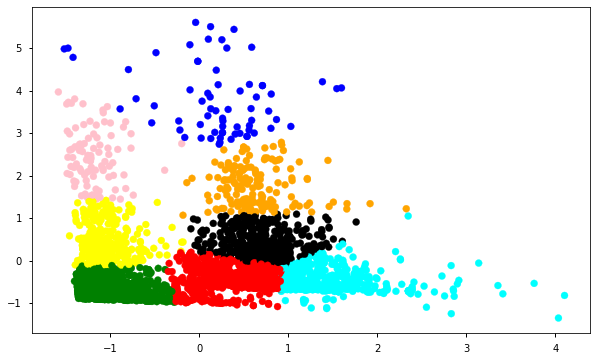
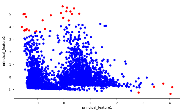
基于聚类的异常检测中强调的假设是我们对数据聚类,正常的数据归属于簇,而异常不属于任何簇或者属于很小的簇。下面我们找出异常并进行可视化。
- 计算每个点和离它最近的聚类中心的距离。最大的那些距离就是异常
- 我们用outliers_fraction给算法提供数据集中离群点比例的信息
- 使用outliers_fraction计算number_of_outliers
- 将threshold设置为离群点间的最短距离
- anomaly1的异常结果包括上述方法的簇(0:正常,1:异常)
- 使用集群视图可视化异常
- 使用时序视图可视化异常
def getDistanceByPoint(data, model):
    distance = pd.Series()
    for i in range(0, len(data)):
        Xa = np.array(data.loc[i])
        Xb = model.cluster_centers_[model.labels_[i]-1]
        distance.set_value(i, np.linalg.norm(Xa-Xb))
    return distance

outliers_fraction = 0.01
distance = getDistanceByPoint(data, kmeans[6])
outlier_num = int(outliers_fraction*len(distance))
threshold = distance.nlargest(outlier_num).min()
df['anomaly'] = (distance >= threshold).astype(int)

fig, ax = plt.subplots(figsize=(10,6))
colors = {0:'blue', 1:'red'}
ax.scatter(df['principal_feature1'], df['principal_feature2'], c=df['anomaly'].apply(lambda x: colors[x]))
plt.xlabel('principal_feature1')
plt.ylabel('principal_feature2')
plt.show()
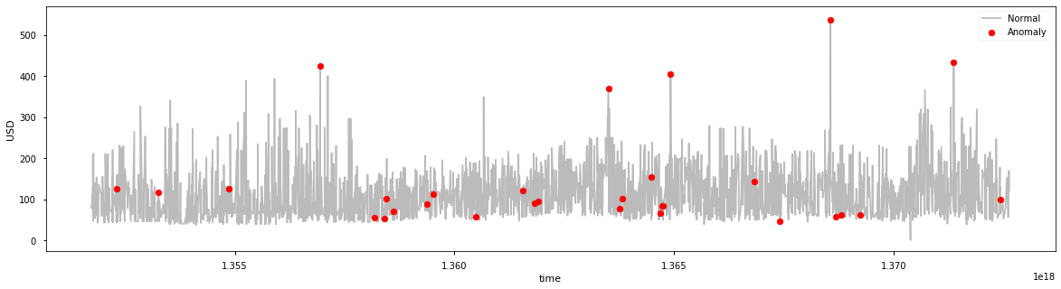
df = df.sort_values('date_time')
df['date_time'] = df.date_time.astype(np.int64)
df['date_time_int'] = df.date_time.astype(np.int64)
# object with anomalies
a = df.loc[df['anomaly'] == 1, ['date_time_int', 'price_usd']]
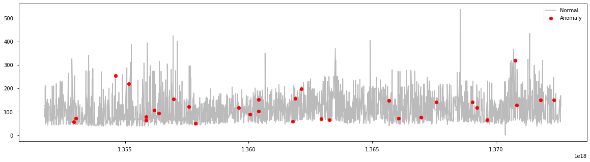
fig, ax = plt.subplots(figsize=(20,5))
ax.plot(df['date_time_int'], df['price_usd'], color='#BBBBBB', label='Normal')
ax.scatter(a['date_time_int'], a['price_usd'], color='red', label='Anomaly', zorder=10)
plt.xlabel('time')
plt.ylabel('USD')
plt.legend()
plt.show()
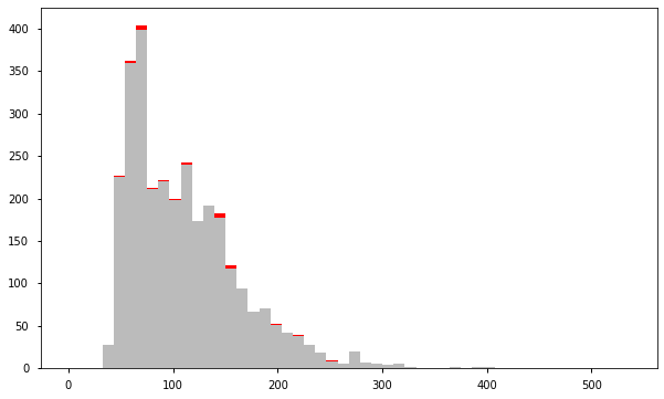
a = df.loc[df['anomaly'] == 0, 'price_usd']
b = df.loc[df['anomaly'] == 1, 'price_usd']

fig, axs = plt.subplots(figsize=(10,6))
axs.hist([a, b], bins=50, stacked=True, color=['#BBBBBB', 'red'])
plt.show()
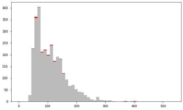
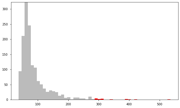
结果表明,k-平均聚类检测到的异常房费要么非常高,要么非常低。
基于孤立森林(IsolationForest)进行异常检测
孤立森林纯粹基于异常值的数量少且取值有异这一情况来进行检测。异常隔离不用度量任何距离或者密度就可以实现。这与基于聚类或者基于距离的算法完全不同。
- 使用IsolationForest模型,设置contamination=outliers_fraction,即这异常的比例
- fit和predict(data)在数据集上执行异常检测,对于正常值返回1,对于异常值返回-1
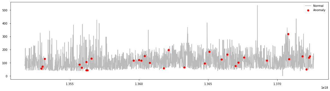
from sklearn.ensemble import IsolationForest

data = df[['price_usd', 'srch_booking_window', 'srch_saturday_night_bool']]
scaler = StandardScaler()
np_scaled = scaler.fit_transform(data)
data = pd.DataFrame(np_scaled)

# Isolationforest
outliers_fraction = 0.01
ifo = IsolationForest(contamination=outliers_fraction)
ifo.fit(data)

df['anomaly1'] = pd.Series(ifo.predict(data))

a = df.loc[df['anomaly1'] == -1, ['date_time_int', 'price_usd']]

fig, ax = plt.subplots(figsize=(20, 5))
ax.plot(df['date_time_int'], df['price_usd'], color='#BBBBBB', label='Normal')
ax.scatter(a['date_time_int'], a['price_usd'], color='red', label='Anomaly', zorder=10)
plt.legend()
plt.show()
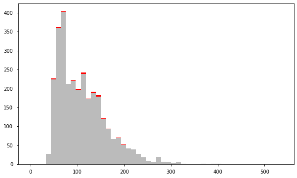
a = df.loc[df['anomaly1'] == 1, 'price_usd']
b = df.loc[df['anomaly1'] == -1, 'price_usd']

fig, ax = plt.subplots(figsize=(10, 6))
ax.hist([a, b], bins=50, stacked=True, color=['#BBBBBB', 'red'])
plt.show()
基于支持向量机的异常检测(OneClassSVM)
SVM和监督学习紧密相连,但是OneClassSVM可以将异常检测当作一个无监督的问题,学得一个决策函数:将新数据归类为与训练数据集相似或者与训练数据集不同:
- 在拟合OneClassSVM模型时,设置nu=outliers_fraction,设置离群值占比
- 指定算法中的核函数类型:rbf。此时SVM使用非线性函数将超空间映射到更高维度中
- predict(data)执行数据分类。会返回+1或者-1,-1代表异常,1代表正常
from sklearn.svm import OneClassSVM

data = df[['price_usd', 'srch_booking_window', 'srch_saturday_night_bool']]
scaler = StandardScaler()
np_scaled = scaler.fit_transform(data)
data = pd.DataFrame(np_scaled)

# Train
osvm = OneClassSVM(nu=outliers_fraction, kernel='rbf', gamma=0.01)
osvm.fit(data)
df['anomaly2'] = pd.Series(osvm.predict(data))

a = df.loc[df['anomaly2'] == -1, ['date_time_int', 'price_usd']]

fig, ax = plt.subplots(figsize=(20, 5))
ax.plot(df['date_time_int'], df['price_usd'], color='#BBBBBB', label='Normal')
ax.scatter(a['date_time_int'], a['price_usd'], color='red', label='Anomaly', zorder=10)
plt.legend()
plt.show()
a = df.loc[df['anomaly2'] == 1, 'price_usd']
b = df.loc[df['anomaly2'] == -1, 'price_usd']

fig, ax = plt.subplots(figsize=(10, 6))
ax.hist([a, b], bins=50, stacked=True, color=['#BBBBBB', 'red'])
plt.show()
基于高斯分布进行异常检测
高斯分布又称为正态分布。假设数据服从正态分布。这个假设并不适用于所有数据集,一旦成立,就能高效地确定离群点。Scikit-Learn的covariance.EllipticEnvelope函数假设全体数据是概率分布的外在表现形式,其背后服从一项多变量高斯分布,以此尝试计算数据数据总体分布的关键参数:
- 创建两个不同的数据集:search_Sat_night、Search_Non_Sat_night。
- 对每个类别使用EllipticEnvelope(高斯分布)。
- 我们设置contamination参数,它是数据集中出现的离群点的比例
- 我们用decision_function来计算给定观测值的决策函数。
- predict(X_train)使用拟合好的模型预测X_train的标签(1表示正常,-1表示异常)
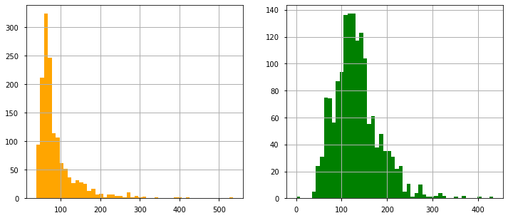
df_class0 = df.loc[df['srch_saturday_night_bool'] == 0, 'price_usd']
df_class1 = df.loc[df['srch_saturday_night_bool'] == 1, 'price_usd']

fig, axs = plt.subplots(1, 2, figsize=(12, 5))
df_class0.hist(ax=axs[0], bins=50, color='orange')
df_class1.hist(ax=axs[1], bins=50, color='green')
 from sklearn.covariance import EllipticEnvelope
envelope = EllipticEnvelope(contamination=outliers_fraction)
x_train = df_class0.values.reshape(-1, 1)
envelope.fit(x_train)
df_class0 = pd.DataFrame(df_class0)
df_class0[‘deviation’] = envelope.decision_function(x_train)
df_class0[‘anomaly’] = envelope.predict(x_train)
df_class = pd.concat([df_class0, df_class1])
df[‘anomaly3’] = df_class[‘anomaly’]
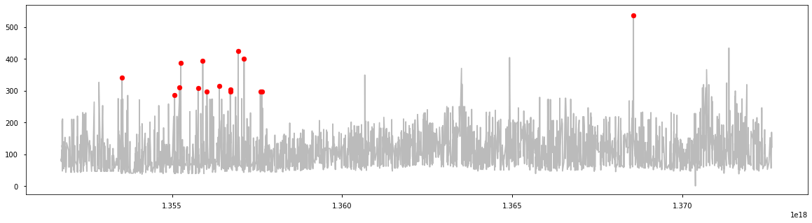
a = df.loc[df[‘anomaly3’] == -1, (‘date_time_int’, ‘price_usd’)]
fig, ax = plt.subplots(figsize=(20, 5))
ax.plot(df[‘date_time_int’], df[‘price_usd’], color=’#BBBBBB’, label=’Normal’)
ax.scatter(a[‘date_time_int’], a[‘price_usd’], color=’red’, label=’Anomaly’, zorder=10)
plt.show()
a = df.loc[df['anomaly3'] == 1, 'price_usd']
b = df.loc[df['anomaly3'] == -1, 'price_usd']

fig, ax = plt.subplots(figsize=(10, 6))
ax.hist([a, b], bins=50, stacked=True, color=['#BBBBBB', 'red'])
plt.show()
基于马尔可夫链(MarkovChain)的异常检测
马尔可夫链可以度量一系列事件发生的概率。我们可以建立一个马尔可夫链,当事件发生时,我们可以用马尔可夫链来度量该序列发生的概率,并用它来检测是否异常。在我们的价格异常检测项目中,我们需要离散化马尔可夫链定义状态下的数据点。我们将使用“price_usd”来定义这个示例的状态,并定义5个级别的值(非常低、低、平均、高、非常高)/(VL、L、A、H、VH)。然后马尔可夫链用状态VL,L,L,A,A,H,H,VH表示。然后,我们可以找到任何新序列发生的概率,然后将稀有序列标记为异常。
from pyemma import msm
# train markov model to get transition matrix
def getTransitionMatrix(df):
df = np.array(df)
model = msm.estimate_markov_model(df, 1)
return model.transition_matrix
# return the success probability of the state change
def successProbabilityMetric(state1, state2, transition_matrix):
proba = 0
for k in range(0, len(transition_matrix)):
if(k != (state2-1)):
proba += transition_matrix[state1-1][k]
return 1-proba
# return the success probability of the whole sequence
def sucessScore(sequence, transition_matrix):
proba = 0
for i in range(1, len(sequence)):
if(i == 1):
proba = successProbabilityMetric(sequence[i-1], sequence[i], transition_matrix)
else:
proba = proba*successProbabilityMetric(sequence[i-1], sequence[i], transition_matrix)
return proba
# return if the sequence is an anomaly considering a threshold
def anomalyElement(sequence, threshold, transition_matrix):
if(sucessScore(sequence, transition_matrix) > threshold):
return 0
else:
return 1
# return a dataframe containing anomaly result for the whole dataset
# choosing a sliding windows size (size of sequence to evaluate) and a threshold
def markovAnomaly(df, windows_size, threshold):
transition_matrix = getTransitionMatrix(df)
real_threshold = threshold**windows_size
df_anomaly = []
for j in range(0, len(df)):
if(j < windows_size):
df_anomaly.append(0)
else:
sequence = df[j-windows_size:j]
sequence = sequence.reset_index(drop=True)
df_anomaly.append(anomalyElement(sequence, real_threshold, transition_matrix))
return df_anomaly
# definition of the different state
x1 = (df['price_usd'] <= 55).astype(int)
x2 = ((df['price_usd'] > 55) & (df['price_usd'] <= 200)).astype(int)
x3 = ((df['price_usd'] > 200) & (df['price_usd'] <= 300)).astype(int)
x4 = ((df['price_usd'] > 300) & (df['price_usd'] <= 400)).astype(int)
x5 = (df['price_usd'] > 400).astype(int)
df_mm = x1 + 2*x2 + 3*x3 + 4*x4 + 5*x5
# getting the anomaly labels for our dataset (evaluating sequence of 5 values and anomaly = less than 20% probable)
df_anomaly = markovAnomaly(df_mm, 5, 0.20)
df_anomaly = pd.Series(df_anomaly)
df['anomaly24'] = df_anomaly
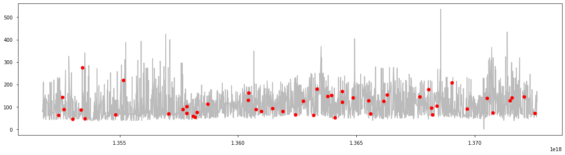
a = df.loc[df['anomaly24'] == 1, ('date_time_int', 'price_usd')] #anomaly
fig, ax = plt.subplots(figsize=(20, 5))
ax.plot(df['date_time_int'], df['price_usd'], color='#BBBBBB', label='Normal')
ax.scatter(a['date_time_int'], a['price_usd'], color='red', label='Anomaly', zorder=10)
plt.show()
a = df.loc[df['anomaly24'] == 0, 'price_usd']
b = df.loc[df['anomaly24'] == 1, 'price_usd']

fig, ax = plt.subplots(figsize=(10, 6))
ax.hist([a, b], bins=50, stacked=True, color=['#BBBBBB', 'red'])
plt.show()
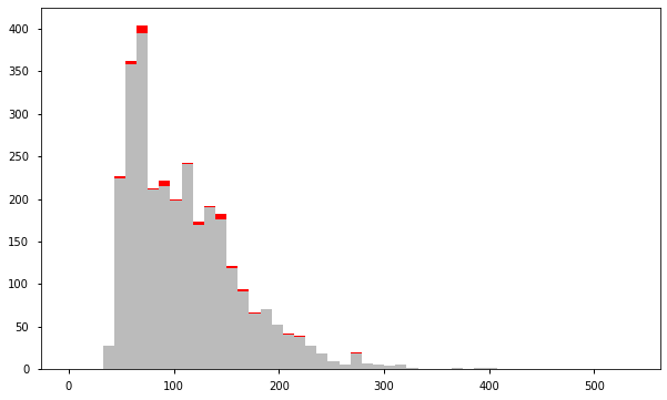
总结
目前使用5种方法进行了异常检测,但是由于是无监督学习,所以不能评估到底哪种方法更合适。需要结合具体的业务场景去分析。从上面的处理过程,个人觉得比较好的是基于高斯分布的异常检测。
参考链接: