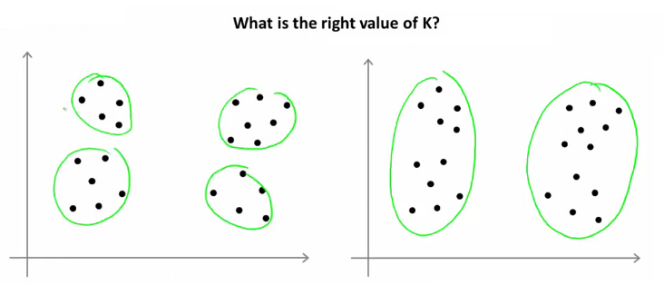
K-Means是一个超级简单的聚类方法,说他简单,主要原因是使用它时只需设置一个K值(设置需要将数据聚成几类)。但问题是,有时候我们拿到的数据根本不知道要分为几类,对于二维的数据,我们还能通过肉眼观察法进行确定,超过二维的数据怎么办?
拍脑袋法
一个非常快速的,拍脑袋的方法是将样本量除以2再开平方出来的值作为K值,具体公式为:
$$K\approx\sqrt{n/2}$$
肘部法则(Elbow Method)
Elbow Method:Elbow意思是手肘,如下图左所示,此种方法适用于K值相对较小的情况,当选择的k值小于真正的时,k每增加1,cost值就会大幅的减小;当选择的k值大于真正的K时,k每增加1,cost值的变化就不会那么明显。这样,正确的k值就会在这个转折点,类似elbow的地方。如下图:
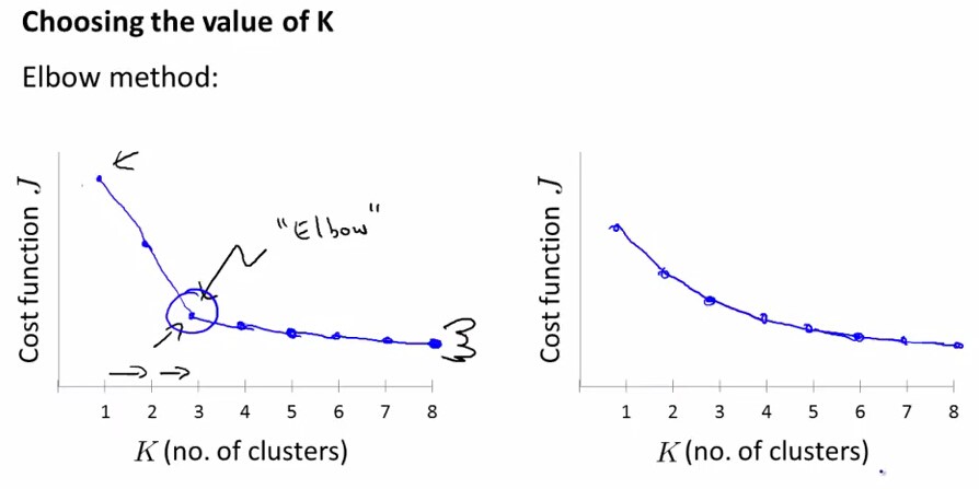
通过画K与cost function的关系曲线图,如左图所示,肘部的值(cost function开始时下降很快,在肘部开始平缓了)做为K值,K=3。并不是所有的问题都可以通过画肘部图来解决,有的问题如右边的那个图,肘点位置不明显(肘点可以是3,4,5),这时就无法确定K值了。故肘部图是可以尝试的一种方法,但是并不是对所有的问题都能画出如左边那么好的图来确定K值。
Elbow Method公式:
$$D_k=\sum_{i=1}^{K}{\sum{dist(x,c_i)^2}}$$
Python实现:
# clustering dataset
# determine k using elbow method

from sklearn.cluster import KMeans
from scipy.spatial.distance import cdist
import numpy as np
import matplotlib.pyplot as plt

x1 = np.array([3, 1, 1, 2, 1, 6, 6, 6, 5, 6, 7, 8, 9, 8, 9, 9, 8])
x2 = np.array([5, 4, 5, 6, 5, 8, 6, 7, 6, 7, 1, 2, 1, 2, 3, 2, 3])

plt.plot()
plt.xlim([0, 10])
plt.ylim([0, 10])
plt.title('Dataset')
plt.scatter(x1, x2)
plt.show()

# create new plot and data
plt.plot()
X = np.array(list(zip(x1, x2))).reshape(len(x1), 2)
colors = ['b', 'g', 'r']
markers = ['o', 'v', 's']

# kmeans determine k
distortions = []
K = range(2, 10)
for k in K:
    kmeanModel = KMeans(n_clusters=k).fit(X)
    distortions.append(sum(np.min(cdist(X, kmeanModel.cluster_centers_, 'euclidean'), axis=1)) / X.shape[0])

# Plot the elbow
plt.plot(K, distortions, 'bx-')
plt.xlabel('k')
plt.ylabel('Distortion')
plt.title('The Elbow Method showing the optimal k')
plt.show()
间隔统计量Gap Statistic
根据肘部法则选择最合适的K值有事并不是那么清晰,因此斯坦福大学的Robert等教授提出了Gap Statistic方法。
这里我们要继续使用上面的$D_k$。Gap Statistic的定义为:
$$Gap_n(k)=E^*_n(log(D_k))-logD_k$$
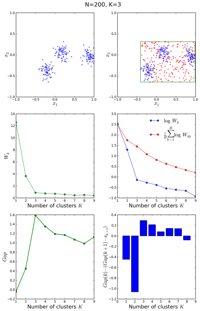
这里${E}(\logD_k)$指的是$logD_k$的期望。这个数值通常通过蒙特卡洛模拟产生,我们在样本里所在的矩形区域中(高维的话就是立方体区域)按照均匀分布随机地产生和原始样本数一样多的随机样本,并对这个随机样本做K-Means,从而得到一个$D_k$。如此往复多次,通常20次,我们可以得到20个$logD_k$。对这20个数值求平均值,就得到了${E}(\logD_k)$的近似值。最终可以计算Gap Statisitc。而Gap statistic取得最大值所对应的K就是最佳的K。
Gap Statistic的基本思路是:引入参考的测值,这个参考值可以有Monte Carlo采样的方法获得。
$$E^*_n(log(D_k))=(1/B)\sum_{b=1}^{B}log(D_{kb}^*)$$
B是sampling的次数。为了修正MC带来的误差,我们计算sk也即标准差来矫正Gap Statistic。
$$w’=(1/B)\sum_{b=1}^{B}log(D^*_{kb})$$
$$sd(k)=\sqrt{(1/B)\sum_b(logD^*_{kb}-w’)^2}$$
$$s_k=\sqrt{\frac{1+B}{B}}sd(k)$$
选择满足$Gap_k>=Gap_{k+1}-s_{k+1}$的最小的k作为最优的聚类个数。下图阐释了Gap Statistic的过程。
Python实现:
import scipy
from scipy.spatial.distance import euclidean
from sklearn.cluster import KMeans as k_means

dst = euclidean

k_means_args_dict = {
    'n_clusters': 0,
    # drastically saves convergence time
    'init': 'k-means++',
    'max_iter': 100,
    'n_init': 1,
    'verbose': False,
    # 'n_jobs': 8
}


def gap(data, refs=None, nrefs=20, ks=range(1, 11)):
    """
    I: NumPy array, reference matrix, number of reference boxes, number of clusters to test
    O: Gaps NumPy array, Ks input list

    Give the list of k-values for which you want to compute the statistic in ks. By Gap Statistic
    from Tibshirani, Walther.
    """
    shape = data.shape

    if not refs:
        tops = data.max(axis=0)
        bottoms = data.min(axis=0)
        dists = scipy.matrix(scipy.diag(tops - bottoms))
        rands = scipy.random.random_sample(size=(shape[0], shape[1], nrefs))
        for i in range(nrefs):
            rands[:, :, i] = rands[:, :, i] * dists + bottoms
    else:
        rands = refs

    gaps = scipy.zeros((len(ks),))

    for (i, k) in enumerate(ks):
        k_means_args_dict['n_clusters'] = k
        kmeans = k_means(**k_means_args_dict)
        kmeans.fit(data)
        (cluster_centers, point_labels) = kmeans.cluster_centers_, kmeans.labels_

        disp = sum(
            [dst(data[current_row_index, :], cluster_centers[point_labels[current_row_index], :]) for current_row_index
            in range(shape[0])])

        refdisps = scipy.zeros((rands.shape[2],))

        for j in range(rands.shape[2]):
            kmeans = k_means(**k_means_args_dict)
            kmeans.fit(rands[:, :, j])
            (cluster_centers, point_labels) = kmeans.cluster_centers_, kmeans.labels_
            refdisps[j] = sum(
                [dst(rands[current_row_index, :, j], cluster_centers[point_labels[current_row_index], :]) for
                current_row_index in range(shape[0])])

        # let k be the index of the array 'gaps'
        gaps[i] = scipy.mean(scipy.log(refdisps)) - scipy.log(disp)

    return ks, gaps
轮廓系数(Silhouette Coefficient)
Silhouette method会衡量对象和所属簇之间的相似度——即内聚性(cohesion)。当把它与其他簇做比较,就称为分离性(separation)。该对比通过silhouette值来实现,后者在[-1,1]范围内。Silhouette值接近1,说明对象与所属簇之间有密切联系;反之则接近-1。若某模型中的一个数据簇,生成的基本是比较高的silhouette值,说明该模型是合适、可接受的。
方法:
1)计算样本i到同簇其他样本的平均距离a(i)。a(i)越小,说明样本i越应该被聚类到该簇。将a(i)称为样本i的簇内不相似度。簇C中所有样本的a(i)均值称为簇C的簇不相似度。
2)计算样本i到其他某簇C(j)的所有样本的平均距离b(ij),称为样本i与簇C(j)的不相似度。定义为样本i的簇间不相似度:b(i)=min{bi1,bi2,…,bik},b(i)越大,说明样本i越不属于其他簇。
3)根据样本i的簇内不相似度ai和簇间不相似度bi,定义样本i的轮廓系数:
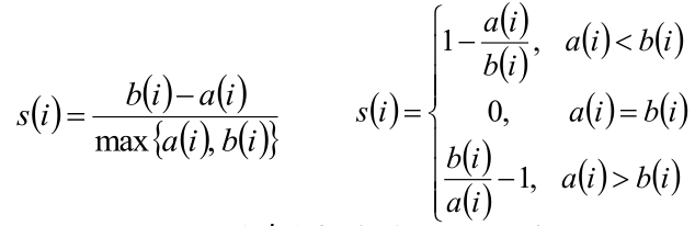
4)判断:
- s(i)接近1,则说明样本i聚类合理
- s(i)接近-1,则说明样本i更应该分类到另外的簇
- 若s(i)近似为0,则说明样本i在两个簇的边界上
所有样本的s(i)的均值称为聚类结果的轮廓系数,是该聚类是否合理、有效的度量。但是,其缺陷是计算复杂度为O(n^2),需要计算距离矩阵,那么当数据量上到百万,甚至千万级别时,计算开销会非常巨大。
Python实现:
import numpy as np
from sklearn.cluster import KMeans
from sklearn import metrics
import matplotlib.pyplot as plt

plt.figure(figsize=(8, 10))
plt.subplot(3, 2, 1)
x1 = np.array([1, 2, 3, 1, 5, 6, 5, 5, 6, 7, 8, 9, 7, 9])
x2 = np.array([1, 3, 2, 2, 8, 6, 7, 6, 7, 1, 2, 1, 1, 3])
X = np.array(list(zip(x1, x2))).reshape(len(x1), 2)
plt.xlim([0, 10])
plt.ylim([0, 10])
plt.title('Sample')
plt.scatter(x1, x2)
colors = ['b', 'g', 'r', 'c', 'm', 'y', 'k', 'b']
markers = ['o', 's', 'D', 'v', '^', 'p', '*', '+']
tests = [2, 3, 4, 5, 8]
subplot_counter = 1
for t in tests:
    subplot_counter += 1
    plt.subplot(3, 2, subplot_counter)
    kmeans_model = KMeans(n_clusters=t).fit(X)
    for i, l in enumerate(kmeans_model.labels_):
        plt.plot(x1[i], x2[i], color=colors[l], marker=markers[l], ls='None')
    plt.xlim([0, 10])
    plt.ylim([0, 10])
    plt.title('K=%s, Silhouette method=%.03f' % (t, metrics.silhouette_score(X, kmeans_model.labels_, metric='euclidean')))
plt.show()
Canopy算法
肘部法则(Elbow Method)和轮廓系数(Silhouette Coefficient)来对k值进行最终的确定,但是这些方法都是属于“事后”判断的,而Canopy算法的作用就在于它是通过事先粗聚类的方式,为k-means算法确定初始聚类中心个数和聚类中心点。
与传统的聚类算法(比如K-Means)不同,Canopy聚类最大的特点是不需要事先指定k值(即clustering的个数),因此具有很大的实际应用价值。与其他聚类算法相比,Canopy聚类虽然精度较低,但其在速度上有很大优势,因此可以使用Canopy聚类先对数据进行“粗”聚类,得到k值,以及大致的k个中心点,再使用K-Means进行进一步“细”聚类。所以Canopy+K-Means这种形式聚类算法聚类效果良好。
 Canopy算法解析:
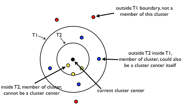
- 原始数据集合 List 按照一定的规则进行排序(这个规则是任意的,但是一旦确定就不再更改),初始距离阈值为 T1、T2,且 T1>T2(T1、T2 的设定可以根据用户的需要,或者使用交叉验证获得)。
- 在 List 中随机挑选一个数据向量 A,使用一个粗糙距离计算方式计算 A 与 List 中其他样本数据向量之间的距离 d。
- 根据第 2 步中的距离 d,把 d 小于 T1 的样本数据向量划到一个 canopy 中,同时把 d 小于 T2 的样本数据向量从候选中心向量名单(这里可以理解为就是 List)中移除。
- 重复第 2、3 步,直到候选中心向量名单为空,即 List 为空,算法结束。
算法原理比较简单,就是对数据进行不断遍历,T2<dis<T1 的可以作为中心名单,dis<T2 的认为与 canopy 太近了,以后不会作为中心点,从 list 中删除,这样的话一个点可能属于多个 canopy。
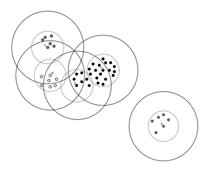
Canopy 效果图如下:
Canopy 算法优势:
- Kmeans 对噪声抗干扰较弱,通过 Canopy 对比较小的 NumPoint 的 Cluster 直接去掉有利于抗干扰。
- Canopy 选择出来的每个 Canopy 的 centerPoint 作为 Kmeans 比较科学。
- 只是针对每个 Canopy 的内容做 Kmeans 聚类,减少相似计算的数量。
Canopy 算法缺点:
- 算法中 T1、T2(T2<T1)的确定问题
Python 实现:
# -*- coding: utf-8 -*-
import math
import random
import numpy as np
import matplotlib.pyplot as plt

class Canopy:
    def __init__(self, dataset):
        self.dataset = dataset
        self.t1 = 0
        self.t2 = 0

    # 设置初始阈值
    def setThreshold(self, t1, t2):
        if t1 > t2:
            self.t1 = t1
            self.t2 = t2
        else:
            print('t1 needs to be larger than t2!')

    # 使用欧式距离进行距离的计算
    def euclideanDistance(self, vec1, vec2):
        return math.sqrt(((vec1 - vec2)**2).sum())

    # 根据当前 dataset 的长度随机选择一个下标
    def getRandIndex(self):
        return random.randint(0, len(self.dataset) - 1)

    def clustering(self):
        if self.t1 == 0:
            print('Please set the threshold.')
        else:
            canopies = []  # 用于存放最终归类结果
            while len(self.dataset) != 0:
                rand_index = self.getRandIndex()
                current_center = self.dataset[rand_index]  # 随机获取一个中心点,定为 P 点
                current_center_list = []  # 初始化 P 点的 canopy 类容器
                delete_list = []  # 初始化 P 点的删除容器
                self.dataset = np.delete(
                    self.dataset, rand_index, 0)  # 删除随机选择的中心点 P
                for datum_j in range(len(self.dataset)):
                    datum = self.dataset[datum_j]
                    distance = self.euclideanDistance(
                        current_center, datum)  # 计算选取的中心点 P 到每个点之间的距离
                    if distance < self.t1:
                        # 若距离小于 t1,则将点归入 P 点的 canopy 类
                        current_center_list.append(datum)
                    if distance < self.t2:
                        delete_list.append(datum_j)  # 若小于 t2 则归入删除容器
                # 根据删除容器的下标,将元素从数据集中删除
                self.dataset = np.delete(self.dataset, delete_list, 0)
                canopies.append((current_center, current_center_list))
            return canopies


def showCanopy(canopies, dataset, t1, t2):
    fig = plt.figure()
    sc = fig.add_subplot(111)
    colors = ['brown', 'green', 'blue', 'y', 'r', 'tan', 'dodgerblue', 'deeppink', 'orangered', 'peru', 'blue', 'y', 'r',
              'gold', 'dimgray', 'darkorange', 'peru', 'blue', 'y', 'r', 'cyan', 'tan', 'orchid', 'peru', 'blue', 'y', 'r', 'sienna']
    markers = ['*', 'h', 'H', '+', 'o', '1', '2', '3', ',', 'v', 'H', '+', '1', '2', '^',
               '<', '>', '.', '4', 'H', '+', '1', '2', 's', 'p', 'x', 'D', 'd', '|', '_']
    for i in range(len(canopies)):
        canopy = canopies[i]
        center = canopy[0]
        components = canopy[1]
        sc.plot(center[0], center[1], marker=markers[i],
                color=colors[i], markersize=10)
        t1_circle = plt.Circle(
            xy=(center[0], center[1]), radius=t1, color='dodgerblue', fill=False)
        t2_circle = plt.Circle(
            xy=(center[0], center[1]), radius=t2, color='skyblue', alpha=0.2)
        sc.add_artist(t1_circle)
        sc.add_artist(t2_circle)
        for component in components:
            sc.plot(component[0], component[1],
                    marker=markers[i], color=colors[i], markersize=1.5)
    maxvalue = np.amax(dataset)
    minvalue = np.amin(dataset)
    plt.xlim(minvalue - t1, maxvalue + t1)
    plt.ylim(minvalue - t1, maxvalue + t1)
    plt.show()


if __name__ == "__main__":
    dataset = np.random.rand(500, 2)  # 随机生成 500 个二维 [0,1) 平面点
    t1 = 0.6
    t2 = 0.4
    gc = Canopy(dataset)
    gc.setThreshold(t1, t2)
    canopies = gc.clustering()
    print('Get %s initial centers.' % len(canopies))
    showCanopy(canopies, dataset, t1, t2)
参考资料:


太有用了