由于Logistic Regression算法复杂度低、容易实现等特点,在工业界中得到广泛使用,如计算广告中的点击率预估等。但是,Logistic Regression算法主要是用于处理二分类问题,若需要处理的是多分类问题,如手写字识别,即识别是{0,1,…,9}中的数字,此时,需要使用能够处理多分类问题的算法。Softmax Regression算法是Logistic Regression算法在多分类问题上的推广,主要用于处理多分类问题,其中,任意两个类之间是线性可分的。
Logistic Regression
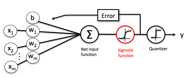
在Logistic回归中比较重要的有两个公式,一个是阶跃函数:
$$h_{\theta}(x)=\frac{1}{1+e^{-\theta^{T}x}}$$
另一个是对应的损失函数:
$$J(\theta)=-\frac{1}{m}\left[\sum_{i=1}^{m}y^{(i)}\log h_{\theta}\left(x^{(i)}\right)+\left(1-y^{(i)}\right)\log\left(1-h_{\theta}\left(x^{(i)}\right)\right)\right]$$
最终,Logistic回归需要求出的是两个概率:$P(y=1|x;\theta)$和$P(y=0|x;\theta)$。具体的Logistic回归的过程可参见“机器学习算法之逻辑回归”。
Softmax Regression
在Logistic回归需要求解的是两个概率,而在Softmax Regression中将不是两个概率,而是k个概率,k表示的是分类的个数。我们需要求出以下的概率值:
$$h_{\theta}\left(x^{(i)}\right)=\left(\begin{array}{c}{P\left(y^{(i)}=1|x^{(i)};\theta\right)}\\{P\left(y^{(i)}=2|x^{(i)};\theta\right)}\\{\cdots}\\{P\left(y^{(i)}=k|x^{(i)};\theta\right)}\end{array}\right)=\frac{1}{\sum_{j=1}^{k}e^{\theta_{j}^{T}x^{(i)}}}\left[\begin{array}{c}{e^{\theta_{1}^{T}x^{(i)}}}\\{e^{\theta_{2}^{T}x^{(i)}}}\\{\cdots}\\{e^{\theta_{k}^{T}x^{(i)}}}\end{array}\right]$$
此时的损失函数为:
$$J(\theta)=-\frac{1}{m}\left[\sum_{i=1}^{m}\sum_{j=1}^{k}I\left\{y^{(i)}=j\right\}\log\frac{e^{\theta_{j}^{T}x^{(i)}}}{\sum_{l=1}^{k}e^{\theta_{l}^{T}x^{(i)}}}\right]$$
其中I{}是一个指示性函数,意思是大括号里的值为真时,该函数的结果为1,否则为0。下面就这几个公式做个解释:
损失函数的由来
概率函数可以表示为:
$$P(y|x;\theta)=\prod_{j=1}^{k}(\frac{e^{\theta_{j}^{T}x}}{\sum_{l=1}^{k}e^{\theta_{l}^{T}x}})^{I\{y=j\}}$$
其似然函数为:
$$L(\theta)=\prod_{i=1}^{m}\prod_{j=1}^{k}(\frac{e^{\theta_{j}^{T}x}}{\sum_{l=1}^{k}e^{\theta_{l}^{T}x}})^{I\{y=j\}}$$
$\log$似然为:
$$l(\theta)=\log L(\theta)=\sum_{i=1}^{m}\sum_{j=1}^{k}I\{y=j\}\log\frac{e^{\theta_{j}^{T}x}}{\sum_{l=1}^{k}e^{\theta_{l}^{T}x}}$$
我们要最大化似然函数,即求$\max l(\theta)$。再转化成损失函数。
对$\log$似然(或者是损失函数)求偏导
为了简单,我们仅取一个样本,则可简单表示为:
$$l(\theta)=\sum_{j=1}^{k}I\{y=j\}\log\frac{e^{\theta_{j}^{T}x}}{\sum_{l=1}^{k}e^{\theta_{l}^{T}x}}$$
对$l(\theta)$求偏导:
$$\frac{\partial l(\theta)}{\partial \theta_{j}^{(m)}}=\sum_{j=1}^{k}I\{y=j\}\left(x^{(m)}-\frac{e^{\theta_{j}^{T}x}}{\sum_{l=1}^{k}e_{l}^{f_{l}}x}\cdot x^{(m)}\right)=[I\{y=j\}-P(y=j|x;\theta)]x^{(m)}$$
其中,表示第维。如Logistic回归中一样,可以使用基于梯度的方法来求解这样的最大化问题。
使用Python实现Softmax Regression
import numpy as np
import random


def load_train_data(input_file):
    feature_data = []
    label_data = []
    with open(input_file) as f:
        for line in f.readlines():
            feature_tmp = []
            feature_tmp.append(1) #偏置项
            lines = line.strip().split("\t")
            for i in range(len(lines)-1):
                feature_tmp.append(float(lines[i]))
            label_data.append(int(lines[-1]))
            feature_data.append(feature_tmp)
    return np.mat(feature_data), np.mat(label_data).T, len(set(label_data))


def load_test_data(num, m):
    """导入测试数据
    :param num:生成的测试样本的个数
    :param m:样本的维数
    :return:生成测试样本
    """
    test_dataset = np.mat(np.ones((num, m)))
    for i in range(num):
        test_dataset[i, 1] = random.random()*6-3 #随机生成[-3,3]之间的随机数
        test_dataset[i, 2] = random.random()*15 #随机生成[0,15]之间是的随机数
    return test_dataset


def cost(err, label_data):
    """计算损失函数值
    :param err:exp的值
    :param label_data:标签的值
    :return:sum_cost/m(float):损失函数的值
    """
    m = np.shape(err)[0]
    sum_cost = 0.0
    for i in range(m):
        if err[i, label_data[i, 0]]/np.sum(err[i, :]) > 0:
            sum_cost -= np.log(err[i, label_data[i, 0]]/np.sum(err[i, :]))
        else:
            sum_cost -= 0
    return sum_cost/m


def gradient_ascent(feature_data, label_data, k, max_cycle, alpha):
    """利用梯度下降法训练Softmax模型
    :param feature_data:特征
    :param label_data:标签
    :param k:类别的个数
    :param max_cycle:最大的迭代次数
    :param alpha:学习率
    :return:weights(mat):权重
    """
    m, n = np.shape(feature_data)
    weights = np.mat(np.ones((n, k))) #权重的初始化
    i = 0
    while i<= max_cycle:
        err = np.exp(feature_data*weights)
        if i % 500 == 0:
            print("\t-----iter:", i, ", cost:", cost(err, label_data))
        row_sum = -err.sum(axis=1)
        row_sum = row_sum.repeat(k, axis=1)
        err = err/row_sum
        for x in range(m):
            err[x, label_data[x, 0]] += 1
        weights = weights + (alpha/m)*feature_data.T*err
        i += 1
    return weights


def save_weights(file_name, weights):
    """保存最终的模型
    :param file_name:保存的文件名
    :param weights:softmax模型
    :return:
    """
    f_w = open(file_name, "w")
    m, n = np.shape(weights)
    for i in range(m):
        w_tmp = []
        for j in range(n):
            w_tmp.append(str(weights[i, j]))
        f_w.write("\t".join(w_tmp)+"\n")
    f_w.close()


def load_weights(weights_path):
    """导入训练好的Softmax模型
    :param weights_path:权重的存储位置
    :return:weights(mat)将权重存到矩阵中
    m(int)权重的行数
    n(int)权重的列数
    """
    with open(weights_path) as f:
        w = []
        for line in f.readlines():
            w_tmp = []
            lines = line.strip().split("\t")
            for x in lines:
                w_tmp.append(float(x))
            w.append(w_tmp)
        weights = np.mat(w)
        m, n = np.shape(weights)
        return weights, m, n


def predict(test_data, weights):
    """利用训练好的Softmax模型对测试数据进行预测
    :param test_data:测试数据的特征
    :param weights:模型的权重
    :return:h.argmax(axis=1)所属的类别
    """
    h = test_data*weights
    return h.argmax(axis=1) #获得所属的类别


def save_result(file_name, result):
    """保存最终的预测结果
    :param file_name:保存最终结果的文件名
    :param result:最终的预测结果
    :return:
    """
    with open(file_name, "w") as f:
        m = np.shape(result)[0]
        for i in range(m):
            f.write(str(result[i, 0])+"\n")


if __name__ == "__main__":
    input_file = "./data/SoftInput.txt"
    feature, label, k = load_train_data(input_file)
    weights = gradient_ascent(feature, label, k, 10000, 0.4) #训练Softmax模型
    save_weights("weights", weights)
    w, m, n = load_weights("weights")
    test_data = load_test_data(4000, m)
    result = predict(test_data, w)
    save_result("result", result)
使用scikit-learn中的Softmax Regression
softmax和Logistic Regression分别适用于多分类和二分类问题,sklearn将这两者放在一起,只需设置相应的参数即可选择分类器与对应的优化算法,需要注意的是loss function是否收敛。
from sklearn.linear_model import LogisticRegression

clf = LogisticRegression(multi_class='ovr', solver='sag')
clf.fit(X_train, y_train)
r = clf.score(X_test, y_test)
参考链接: