在前面介绍的DBSCAN算法中,有两个初始参数Eps(邻域半径)和minPts(Eps邻域最小点数)需要手动设置,并且聚类的结果对这两个参数的取值非常敏感,不同的取值将产生不同的聚类结果。为了克服DBSCAN算法这一缺点,提出了OPTICS算法(Ordering Points to identify the clustering structure),翻译过来就是,对点排序以此来确定簇结构。
OPTICS是对DBSCAN的一个扩展算法。该算法可以让算法对半径Eps不再敏感。只要确定minPts的值,半径Eps的轻微变化,并不会影响聚类结果。OPTICS并不显示的产生结果类簇,而是为聚类分析生成一个增广的簇排序(比如,以可达距离为纵轴,样本点输出次序为横轴的坐标图),这个排序代表了各样本点基于密度的聚类结构。它包含的信息等价于从一个广泛的参数设置所获得的基于密度的聚类,换句话说,从这个排序中可以得到基于任何参数Eps和minPts的DBSCAN算法的聚类结果。
核心距离与可达距离
要搞清楚OPTICS算法,需要搞清楚2个新的定义:核心距离和可达距离。
核心距离
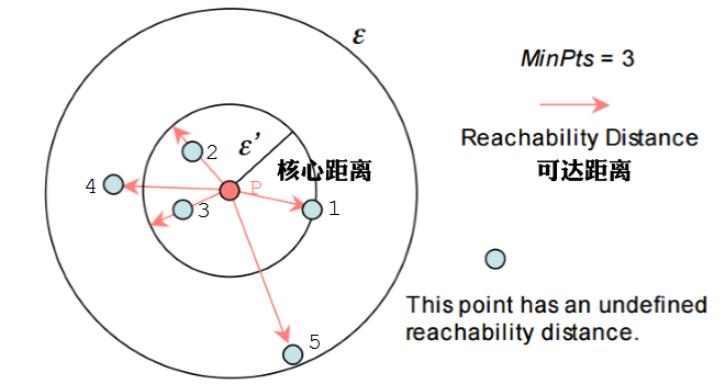
一个对象p的核心距离是使得其成为核心对象的最小半径,如果p不是核心点,其可达距离没有定义。即对于集合M而言,假设让其中x点作为核心,找到以x点为圆心,且刚好满足最小邻点数minPts的最外层的一个点为x’,则x点到x’点的距离称为核心距离。
$$cd(x)=\begin{cases}UNDEFINED,& \text{if}{|N_{\epsilon}(x)|<\mathcal{M}}\\d(x,N_{\epsilon}^{\mathcal{M}}(x),&\text{if}{|N_{\epsilon}(x)|\ge\mathcal{M}}\end{cases}$$
可达距离
可达距离是根据核心距离来定义的。对于核心点x的邻点x1、x2、…xn而言,如果他们到点x的距离大于点x’的核心距离,则其可达距离为该点到点x的实际距离;如果他们到点x的距离核心距离小于点x’的核心距离的话,则其可达距离就是点x的核心距离,即在x’以内的点到x的距离都以此核心距离来记录。
$$rd(y,x)=\begin{cases}UNDEFINED & \text{if}{|N_{\epsilon}(x)|<\mathcal{M}}\\max\{cd(x),d(x,y)\}& \text{if}{|N_{\epsilon}(x)|\ge\mathcal{M}}\end{cases}$$
举例,下图中假设minPts=3,半径是ε。那么P点的核心距离是d(1,P),点2的可达距离是d(1,P),点3的可达距离也是d(1,P),点4的可达距离则是d(4,P)的距离。
OPTICS算法描述
输入:样本集D,邻域半径ε,给定点在ε领域内成为核心对象的最小领域点数MinPts
输出:具有可达距离信息的样本点输出排序
方法:
- 创建两个队列,有序队列和结果队列。(有序队列用来存储核心对象及其该核心对象的直接可达对象,并按可达距离升序排列;结果队列用来存储样本点的输出次序。你可以把有序队列里面放的理解为待处理的数据,而结果队列里放的是已经处理完的数据)。
- 如果所有样本集D中所有点都处理完毕,则算法结束。否则,选择一个未处理(即不在结果队列中)且为核心对象的样本点,找到其所有直接密度可达样本点,如过该样本点不存在于结果队列中,则将其放入有序队列中,并按可达距离排序
- 如果有序队列为空,则跳至步骤2(重新选取处理数据)。否则,从有序队列中取出第一个样本点(即可达距离最小的样本点)进行拓展,并将取出的样本点保存至结果队列中(如果它不存在结果队列当中的话)。然后进行下面的处理。
- 判断该拓展点是否是核心对象,如果不是,回到步骤3(因为它不是核心对象,所以无法进行扩展了。那么就回到步骤3里面,取最小的。这里要注意,第二次取不是取第二小的,因为第一小的已经放到了结果队列中了,所以第二小的就变成第一小的了。)。如果该点是核心对象,则找到该拓展点所有的直接密度可达点。
- 判断该直接密度可达样本点是否已经存在结果队列,是则不处理,否则下一步。
- 如果有序队列中已经存在该直接密度可达点,如果此时新的可达距离小于旧的可达距离,则用新可达距离取代旧可达距离,有序队列重新排序(因为一个对象可能直接由多个核心对象可达,因此,可达距离近的肯定是更好的选择)。
- 如果有序队列中不存在该直接密度可达样本点,则插入该点,并对有序队列重新排序。
- 迭代2,3。
- 算法结束,输出结果队列中的有序样本点。
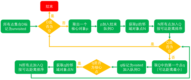
上面的的描述可能让你听了云里雾里的,接下来我们以流程图的方式看下执行过程:
- D: 待聚类的集合
- Q: 有序队列,元素按照可达距离排序,可达距离最小的在队首
- O: 结果队列,最后输出结果的点集的有序队列
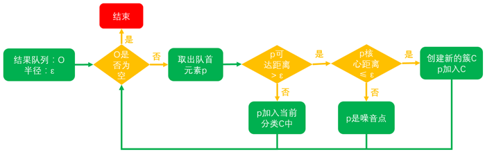
得到结果队列后,使用如下算法得到最终的聚类结果:
- 从结果队列中按顺序取出点,如果该点的可达距离不大于给定半径ε,则该点属于当前类别,否则至步骤2
- 如果该点的核心距离大于给定半径ε,则该点为噪声,可以忽略,否则该点属于新的聚类,跳至步骤1
- 结果队列遍历结束,则算法结束
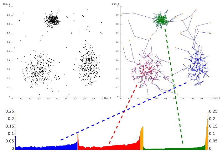
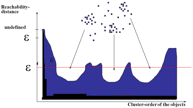
上面的算法处理完后,我们得到了输出结果序列,每个节点的可达距离和核心距离。我们以可达距离为纵轴,样本点输出次序为横轴进行可视化:
其中:
- X轴代表OPTICS算法处理点的顺序,Y轴代表可达距离。
- 簇在坐标轴中表述为山谷,并且山谷越深,簇越紧密
- 黄色代表的是噪声,它们不形成任何凹陷。
当你需要提取聚集的时候,参考Y轴和图像,自己设定一个阀值就可以提取聚集了。再来一张凹陷明显的:
OPTICS的核心思想:
- 较稠密簇中的对象在簇排序中相互靠近
- 一个对象的最小可达距离给出了一个对象连接到一个稠密簇的最短路径
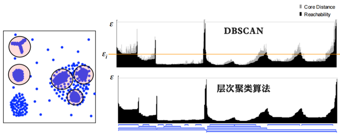
每个团簇的深浅代表了团簇的紧密程度,我们可以在这基础上采用DBSCAN(选取最优的Eps)或层次聚类方法对数据进行聚类。
基于OPTICS算法扩展有很多,比如:
- OPTICS-OF用来检测异常值(Outliar Detection)
- DeLi-Clu 算法来消除 eps 参数,提供比 OPTICS 更好的性能指标
- HiSC 算法将其应用到 Subspace Clustering
- HiCO 应用到相关聚类 (Correlation Clustering) 上
- 基于 HiSC 改进的 DiSH 能够找到更加复杂的簇结构
OPTICS 邻域半径 ε
OPTICS 算法不是为了解决 DBSACN 的参数设置问题吗?为什么算法中还需要输入参数 ε 和minPts?其实这里的 ε 和minPts 只是起到算法辅助作用,也就是说 ε 和minPts 的细微变化并不会影响到样本点的相对输出顺序,这对我们分析聚类结果是没有任何影响。
为什么说 OPTICS 算法对于 ε 不敏感,在算法参数上还要输入 ε 呢?
因为基于密度的聚类算法需要确定哪些点是核心点,哪些是躁点。所以为了这个目的,需要有个半径 ε。所以 ε 是必须给定的。
为什么当 ε 发生了变化,根据输出队列 O 还是可以得到新的分类?
在 OPTICS 算法中 minPts 并没有发生变化,虽然给定了 ε,但最终得到的不是直接的分类结果,而是在这个 ε 和 minPts 下的有序队列,以及所有点的核心距离和可达距离。我们使用另外一个小的算法从队列中得到分类。简而言之:OPTICS 算法通过给定一个 ε 值和 minPts,计算出来的所有小于等于 ε 的情况的特征,最后利用这些特征,做一些简要的逻辑计算就可以得到分类。在对结果队列 O 的处理中,判断核心距离 ≤ ε’ 这实则已经是在判断 P 是否为新半径 ε’ 下的核心点了。所以 ε 发生了变化,核心点即使变化了也没关系,在 O 的处理中已经照顾到了,不是核心点的元素一定会被认定为躁点。保证了分类的正确性。
综上所述,OPTICS 可以在minPts 固定的前提下,对于任意的 ε’ (其中 ε’ 小于等于 ε) 都可以直接经过简单的计算得到新的聚类结果。
OPTICS算法的Python 实现
#https://gist.github.com/ryangomba/1724881
import math
from functools import reduce

class Point:
    def __init__(self, latitude, longitude):
        self.latitude = latitude
        self.longitude = longitude
        self.cd = None # core distance
        self.rd = None # reachability distance
        self.processed = False # has this point been processed?

    # calculate the distance between any two points on earth
    def distance(self, point):
        # convert coordinates to radians
        p1_lat, p1_lon, p2_lat, p2_lon = [math.radians(c) for c in
        (self.latitude, self.longitude, point.latitude, point.longitude)]

        numerator = math.sqrt(
            math.pow(math.cos(p2_lat) * math.sin(p2_lon - p1_lon), 2) +
            math.pow(
                math.cos(p1_lat) * math.sin(p2_lat) -
                math.sin(p1_lat) * math.cos(p2_lat) *
                math.cos(p2_lon - p1_lon), 2))

        denominator = (
            math.sin(p1_lat) * math.sin(p2_lat) +
            math.cos(p1_lat) * math.cos(p2_lat) *
            math.cos(p2_lon - p1_lon))

        # convert distance from radians to meters
        # note: earth's radius ~6372800 meters

        return math.atan2(numerator, denominator) * 6372800

    # point as GeoJSON
    def to_geo_json_dict(self, properties=None):
        return {
            'type': 'Feature',
            'geometry': {
                'type': 'Point',
                'coordinates': [
                    self.longitude,
                    self.latitude,
                ]
            },
            'properties': properties,
        }

    def __repr__(self):
        return '(%f, %f)' % (self.latitude, self.longitude)


class Cluster:
    def __init__(self, points):
        self.points = points

    # calculate the centroid for the cluster
    def centroid(self):
        return Point(sum([p.latitude for p in self.points]) / len(self.points),
            sum([p.longitude for p in self.points]) / len(self.points))

    # calculate the region (centroid, bounding radius) for the cluster
    def region(self):
        centroid = self.centroid()
        radius = reduce(lambda r, p: max(r, p.distance(centroid)), self.points)
        return centroid, radius


    # cluster as GeoJSON
    def to_geo_json_dict(self, user_properties=None):
        center, radius = self.region()
        properties = {'radius': radius}
        if user_properties: properties.update(user_properties)

        return {
            'type': 'Feature',
            'geometry': {
                'type': 'Point',
                'coordinates': [
                    center.longitude,
                    center.latitude,
                ]
            },
            'properties': properties,
        }


class Optics:
    def __init__(self, points, max_radius, min_cluster_size):
        self.points = points
        self.max_radius = max_radius # maximum radius to consider
        self.min_cluster_size = min_cluster_size # minimum points in cluster


    # get ready for a clustering run
    def _setup(self):
        for p in self.points:
            p.rd = None
            p.processed = False
        self.unprocessed = [p for p in self.points]
        self.ordered = []


    # distance from a point to its nth neighbor (n = min_cluser_size)
    def _core_distance(self, point, neighbors):
        if point.cd is not None: return point.cd
        if len(neighbors) >= self.min_cluster_size - 1:
            sorted_neighbors = sorted([n.distance(point) for n in neighbors])
            point.cd = sorted_neighbors[self.min_cluster_size - 2]
            return point.cd

    # neighbors for a point within max_radius
    def _neighbors(self, point):
        return [p for p in self.points if p is not point and
            p.distance(point) <= self.max_radius]


    # mark a point as processed
    def _processed(self, point):

        point.processed = True
        self.unprocessed.remove(point)
        self.ordered.append(point)

    # update seeds if a smaller reachability distance is found
    def _update(self, neighbors, point, seeds):
        # for each of point's unprocessed neighbors n...
        for n in [n for n in neighbors if not n.processed]:
            # find new reachability distance new_rd
            # if rd is null, keep new_rd and add n to the seed list
            # otherwise if new_rd< old rd, update rd
            new_rd = max(point.cd, point.distance(n))
            if n.rd is None:
                n.rd = new_rd
                seeds.append(n)
            elif new_rd< n.rd:
                n.rd = new_rd


    # run the OPTICS algorithm
    def run(self):
        self._setup()
        # for each unprocessed point (p)...
        while self.unprocessed:
            point = self.unprocessed[0]
            # mark p as processed
            # find p's neighbors
            self._processed(point)
            point_neighbors = self._neighbors(point)
            # if p has a core_distance, i.e has min_cluster_size - 1 neighbors
            if self._core_distance(point, point_neighbors) is not None:
                # update reachability_distance for each unprocessed neighbor
                seeds = []
                self._update(point_neighbors, point, seeds)
                # as long as we have unprocessed neighbors...
                while(seeds):
                    # find the neighbor n with smallest reachability distance
                    seeds.sort(key=lambda n: n.rd)n = seeds.pop(0)
# mark as processed
# find n's neighbors
self._processed(n)
n_neighbors = self._neighbors(n)
# if p has a core_distance...
if self._core_distance(n, n_neighbors) is not None:
    # update reachability_distance for each of n's neighbors
    self._update(n_neighbors, n, seeds)
# when all points have been processed
# return the ordered list
return self.ordered

#--------------------------------------------------------------------------
def cluster(self, cluster_threshold):
    clusters = []
    separators = []
    for i in range(len(self.ordered)):
        this_i = i
        next_i = i + 1
        this_p = self.ordered[i]
        this_rd = this_p.rd if this_p.rd else float('infinity')
        # use an upper limit to separate the clusters
        if this_rd > cluster_threshold:
            separators.append(this_i)
    separators.append(len(self.ordered))
    for i in range(len(separators) - 1):
        start = separators[i]
        end = separators[i + 1]
        if end - start >= self.min_cluster_size:
            clusters.append(Cluster(self.ordered[start:end]))
    return clusters


if __name__ == "__main__":
    # LOAD SOME POINTS
    points = [
        Point(37.769006, -122.429299),  # cluster #1
        Point(37.769044, -122.429130),  # cluster #1
        Point(37.768775, -122.429092),  # cluster #1
        Point(37.776299, -122.424249),  # cluster #2
        Point(37.776265, -122.424657),  # cluster #2
    ]

    optics = Optics(points, 100, 2)  # 100m radius for neighbor consideration, cluster size >= 2 points
    optics.run()  # run the algorithm
    clusters = optics.cluster(50)  # 50m threshold for clustering

    for cluster in clusters:
        print(cluster.points)
其他参考链接:
- https://en.wikipedia.org/wiki/OPTICS_algorithm
- https://github.com/marionleborgne/optics-demo
- https://github.com/captainsafia/cranberry
- https://github.com/mannmann2/Density-Based-Clustering
- https://github.com/inftechweu/optics
- https://github.com/aonghus/optics-cluster
- https://github.com/dvida/cyoptics-clustering


这么好的文章,为啥没人看
请问第一个加入的核心点,哪里会有可达距离呢?第一个加入到了结果队列,那之后就不会再处理他了啊
第一个加入的点,可达距离是none,在cluster中,如果他是核心点,就形成一个聚类,否则就是噪音点,因此有没有可达距离就无所谓了
写的真好,尤其是插图,解释的很到位
你好,OPTICS 聚类适用于n维向量吗
我没处理过,应该支持的
在OPTICS原文中,从原始点集中提取的并不是核心对象,而是依次取数据点,并输出到结果队列中。区别是核心对象及其密度直达点会经过orderseeds处理再输出到结果队列中。但是几乎所有的博主包括您,从原始点集中取出的都是核心对象,这让我很迷惑。还请指教
您好,请问下为什么山谷图中的每个簇中的核心对象的可达距离都是从低到高,再到低。
学习了,写得非常清楚!