因果推断核心概念
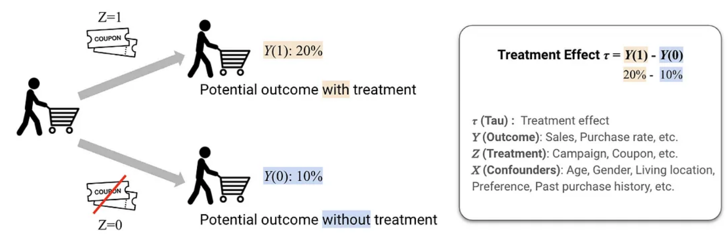
我们将通过一个贯穿始终的简单例子来讲解:评估一个广告(比如一封营销邮件)对用户购买行为的影响。
- 干预(Treatment): 发送营销邮件。
- W = 1:用户被分配到处理组(计划发送邮件)。
- W = 0:用户被分配到对照组(计划不发送邮件)。
- 结果(Outcome): 是否购买。Y = 1(购买),Y = 0(未购买)。
- 核心问题:我们关心的不是“收到邮件的用户购买率有多高”,而是“邮件导致了多少额外的购买”?这就是因果效应。
ATE – 平均处理效应 (Average Treatment Effect)
定义:干预(Treatment)对整个研究人群的平均影响。它回答了“如果我们对所有人施加干预,相比于对所有人都不施加干预,平均结果会差多少?”
公式:ATE = E[Y(1) – Y(0)] = E[Y(1)] – E[Y(0)]
- Y(1):如果接受处理后的潜在结果。
- Y(0):如果未接受处理后的潜在结果。
计算:在完美随机实验中(即分组是随机的),ATE可以简单地估算为:
ATE = (处理组购买率) – (对照组购买率)
例子:
- 处理组(收到邮件)的购买率 = 12%
- 对照组(未收邮件)的购买率 = 8%
- ATE = 12% – 8% = 4%
- 结论:这封营销邮件使得整个用户群体的购买率平均提升了4个百分点。
重要性:ATE是因果推断中最基础、最广泛关注的指标,它给出了干预的整体效果。
ATT – 处理组的平均处理效应 (Average Treatment Effect on the Treated)
定义:干预(Treatment)对实际接受了处理的人群的平均影响。它回答了“对那些实际被处理的人,处理比不处理平均多带来了多少效果?”
公式:ATT = E[Y(1) – Y(0) | W = 1]
与ATE的区别:
- ATE关心的是“对所有人的平均效果”。
- ATT关心的是“对被处理的人的平均效果”。
例子:继续使用邮件营销的例子。假设有些用户邮箱已失效,邮件被退回,他们实际上并未“暴露”在干预下。
- 处理组中实际收到邮件的用户购买率 = 15%
- 假设我们能知道,如果这些同样的人没收到邮件,他们的购买率会是 9%
- ATT = 15% – 9% = 6%
- 结论:这封邮件对那些实际收到它的人,平均产生了6个百分点的购买提升。
重要性:当我们更关心干预对“被触达”群体的效果时(例如计算已花费成本的回报率),ATT比ATE更具参考价值。在观察性研究中,ATT通常比ATE更容易估计。
CATE – 条件平均处理效应 (Conditional Average Treatment Effect)
定义:干预对具有特定特征(X)的子人群的平均影响。它是Uplift Modeling(增量建模)的核心目标。
公式:CATE = E[Y(1) – Y(0) | X = x]
- X是特征变量,比如用户年龄、历史消费等。
与ATE/ATT的区别:
- ATE/ATT给出一个单一的平均值。
- CATE允许效应因人而异,它输出的是一个关于特征 X的函数。
例子:我们想知道邮件对“年轻用户”和“老用户”的效果是否不同。
- 对特征 X(年龄 < 30)的子人群计算:CATE_年轻 = (年轻处理组购买率) – (年轻对照组购买率) = 15% – 5% = 10%
- 对特征 X(年龄 ≥ 30)的子人群计算:CATE_年长 = (年长处理组购买率) – (年长对照组购买率) = 6% – 7% = -1%
- 结论:营销邮件对年轻用户非常有效,平均提升10个百分点的购买率;但对年长用户略有负面效果。因此,最优策略是只给年轻用户发送邮件。
重要性:CATE是实现个性化策略(精准营销、个性化治疗等)的理论基础。CausalML中的模型(如Meta-Learners, Uplift Trees)主要就是为了预测CATE。
ITT – 意向性处理效应 (Intent-to-Treat Effect)
定义:基于最初的干预分配(而不是实际接受情况)来分析效果。它是ATE的一个特例,衡量的是“执行策略”本身的效果。
计算:ITT = E[Y | W=1] – E[Y | W=0](注意:这里只看初始分配 W)
例子:在邮件实验中,即使分配了邮件但有些没发送成功(邮箱错误),我们依然按最初分配的组别来分析:
- 所有被分配到处理组的用户(包括没收到邮件的)购买率 = 10%
- 所有被分配到对照组的用户购买率 = 8%
- ITT = 10% – 8% = 2%
- 结论:“执行发送邮件这个策略”平均为整个群体带来了2个百分点的购买提升。
重要性:ITT非常稳健,因为它严格遵守随机分配,避免了因“未依从”(如邮件发送失败)带来的混淆。它衡量的是策略的执行效果,而不是治疗本身的生物学或心理学效果。
TOT/LATE – 处理效应与局部平均处理效应 (Effect of Treatment on the Treated / Local Average Treatment Effect)
问题背景:当存在非依从性时(即分配了但未接受处理,如 W=1但未曝光),直接比较 Y会产生偏差。我们需要估计实际接受处理的影响。
工具变量法:为了解决非依从性问题,我们将初始分配 Z(即Treatment) 作为一个工具变量(IV),来估计实际处理 D(即Exposure) 对结果 Y的影响。
TOT/LATE定义:工具变量法估计出的效应,代表的是对依从者(Compliers)的平均效应。依从者是指那些行为完全由初始分配决定的人(即 Z=1则 D=1, Z=0则 D=0)。
计算(Wald估计量):LATE = (E[Y | Z=1] – E[Y | Z=0]) / (E[D | Z=1] – E[D | Z=0])
例子(对应Criteo数据集):
- Z(工具变量): treatment(计划分配)
- D(实际处理): exposure(实际曝光)
- Y(结果): conversion(转化)
- 计算:
- 分子:(分配至处理组的用户的转化率) – (分配至对照组的用户的转化率) = ITT
- 分母:(分配至处理组的用户的广告曝光率) – (分配至对照组的用户的广告曝光率)
- 假设:
- 处理组转化率 (Y|Z=1) = 12%,对照组转化率 (Y|Z=0) = 8% -> 分子 ITT = 4%
- 处理组曝光率 (D|Z=1) = 80%(有20%的人没加载出广告),对照组曝光率 (D|Z=0) = 5%(有5%的人通过其他途径看到了广告) -> 分母 = 80% – 5% = 75%
- LATE = 4% / 75% ≈ 5.33%
- 结论:广告曝光对那些依从者(即:被分配看广告且成功看到的人 vs 被分配不看广告就真的没看到的人)的真实因果效应是提升33个百分点的转化率。
重要性:LATE提供了一个在存在非依从性的情况下,估计实际处理效应的有效方法。它比ITT更接近“治疗”的纯效果,但需要注意的是,它只适用于“依从者”这个子群体。
总结与对比
因果推断核心概念总结与对比表
| 概念 | 英文全称 | 核心问题 | 公式/估算 | 特点与应用场景 |
| ATE | Average Treatment Effect | 干预对整个目标群体的平均效果? | ATE = E[Y(1) – Y(0)] | 最基础的指标,用于评估干预的整体价值。 |
| ATT | Average Treatment Effect on the Treated | 干预对实际接受了处理的人群的平均效果? | ATT = E[Y(1) – Y(0)|W=1] | 关注干预对实际触达群体的效果,常用于计算投资回报率(ROI)。 |
| CATE | Conditional Average Treatment Effect | 干预对具有特定特征的子人群的平均效果? | CATE = E[Y(1) – Y(0)|X=x] | 个性化策略的核心,Uplift Modeling的目标,用于识别异质性效应。 |
| ITT | Intent-to-Treat Effect | 执行分配策略本身(而非实际处理)的平均效果? | ITT = E[Y|Z=1] – E[Y|Z=0] | 衡量策略执行的效果,非常稳健,严格遵守随机分配原则。 |
| LATE | Local Average Treatment Effect | 干预对依从者(其行为完全由初始分配决定的人)的平均效果? | LATE=\frac{E[Y|Z=1]-E[Y|Z=0]}{E[D|Z=1]-E[D|Z=0]} | 使用工具变量法(IV) 估计,用于解决非依从性问题,估算实际处理的“纯净”效应。 |
注:符号说明
- Y(1), Y(0): 潜在结果(Potential Outcomes)
- W: 处理指示变量(Treatment Indicator)
- Z: 工具变量(Instrumental Variable),通常是初始分配
- D: 实际接受的处理(Actual Treatment)
- X: 协变量/特征(Covariates/Features)
CausalML简介
CausalML 是一个基于 Python 的开源工具包,它巧妙地将机器学习的预测能力与因果推断的逻辑框架结合在一起,旨在从数据中识别出真正的因果关系,而不仅仅是相关关系。

项目概览
CausalML 的核心任务是估计干预措施(例如发放优惠券、投放广告)的因果效应,特别关注于条件平均处理效应(CATE) 或个体处理效应(ITE)。这意味着它不仅能回答“这个广告活动平均能提升多少销售额?”,更能回答“向哪位特定用户投放这个广告,效果最好?”,从而实现真正的个性化决策。
该项目最初由 Uber 的数据科学团队开发,用以解决其实际的业务问题,之后开源并持续维护,目前已成为因果机器学习领域一个非常受欢迎的工具。
核心功能与方法
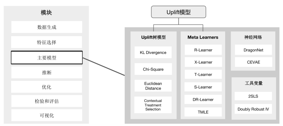
CausalML 作为一个功能丰富的因果推断工具包,提供了多种主流算法来估计干预措施的因果效应。为了帮助你快速了解其算法体系,下面这个表格汇总了核心的算法类别及其代表方法。
| 算法类别 | 代表方法 | 主要特点 / 适用场景 |
| Meta-Learners(元学习器) | S-Learner, T-Learner, X-Learner, R-Learner, DR-Learner | 框架灵活,可以复用现有的机器学习模型(如线性模型、XGBoost等)来估计条件平均处理效应(CATE) |
| 基于树的算法 | Uplift Random Forests (基于KL散度、欧氏距离、卡方), Contextual Treatment Selection (CTS) Trees, Causal Forest | 专门为因果推断设计,通过特定的分裂准则(如提升差异)直接识别对干预敏感的群体 |
| 工具变量算法 | 两阶段最小二乘法 (2SLS), 双稳健工具变量学习器 (DRIV) | 适用于存在未观测混杂因素的情况,需要有一个有效的工具变量(Instrumental Variable) |
| 基于神经网络的方法 | CEVAE (Causal Effect Variational Autoencoder), DragonNet | 利用神经网络的强大表示能力处理复杂的非线性关系和高维数据 |
| 处理效果优化算法 | 反事实单元选择, 反事实价值估计器 | 超越效应估计,直接用于决策优化,例如在营销中最大化投资回报率(ROI) |
基于树的算法 (Tree-based algorithms)
这类算法专门为估计异质性处理效应(HTE)或提升(Uplift)而设计,通过改进决策树的分裂准则来直接优化因果效应的识别。
基于分布差异的森林:
- KL 散度提升随机森林:使用KL散度来衡量干预组和对照组在节点中的分布差异,并以此作为分裂准则。
- 欧氏距离提升随机森林:使用欧氏距离作为分布差异的度量。
- 卡方散度提升随机森林:使用卡方散度作为分布差异的度量。
基于特定准则的森林:
- 上下文处理选择提升随机森林:专注于识别在不同上下文(特征)下最优的处理方案。
- ΔΔP 准则提升随机森林:适用于二分树和二分类问题,直接优化处理组和对照组之间响应率之差。
- IDDP 准则提升随机森林:同样适用于二分树和二分类问题。
经典因果树:
- 交互树:适用于二分树和二分类问题,用于识别处理效应异质性。
- 因果推断树:适用于二分树和二分类问题,是因果推断中的基础树模型。
元学习器算法 (Meta-learner algorithms)
这类方法将因果估计问题转化为标准的有监督学习问题,可以灵活地套用任何机器学习模型(如XGBoost、随机森林、线性模型等)作为其基学习器。
- S-Learner:将处理指示变量作为一个特征,训练单个模型。
- T-Learner:为处理组和对照组分别训练两个独立的模型。
- X-Learner:一种更复杂的元学习器,结合了T-Learner的思想并进行交叉估计,通常在处理效应存在异质性时表现更好。
- R-Learner:基于稳健损失函数和交叉拟合的框架,旨在减少偏差和过拟合。
- 双稳健学习器:结合了处理倾向评分和结果回归模型,只要两者中有一个估计正确,就能得到无偏的效应估计,增强了模型的稳健性。
工具变量算法 (Instrumental variables algorithms)
这类方法用于处理存在未观测混杂因子的情况,但需要一个有效的工具变量。
- 两阶段最小二乘法:最经典的工具变量方法,通过两个阶段的回归来估计因果效应。
- 双稳健工具变量学习器:将工具变量法的思想与双稳健估计相结合,提高了估计的稳健性。
基于神经网络的算法 (Neural network based algorithms)
利用深度学习的强大表示能力来处理复杂的非线性关系和高度数据。
- CEVAE:因果效应变分自编码器,一种结合了变分推理和神经网络的方法,适用于存在未观测混淆因子的场景。
- DragonNet:一种专门的神经网络结构,通过自适应参数估计来提高因果效应估计的效率和精度。
处理效果优化算法 (Treatment optimization algorithms)
这类方法超越了单纯的效应估计,直接聚焦于做出最优决策。
- 反事实单元选择:用于识别哪些个体单元最应该接受处理,以最大化整体效果(例如,选择哪些客户进行营销以最大化ROI)。
- 反事实价值估计器:用于估计在不同处理决策下所能带来的预期价值,从而选择价值最大的决策。
总结与选择指南
为了更直观地展示这些算法的特点和适用场景,可以参考以下表格:
| 算法类别 | 核心思想 | 典型应用场景 | 注意事项 |
| 基于树的算法 | 直接优化因果分裂准则,识别异质性群体 | 精准营销、用户分群、寻找敏感人群 | 部分算法仅支持二分类问题 |
| 元学习器 | 将因果问题转化为预测问题,复用现有ML模型 | 通用性强,可作为大部分因果问题的基线模型 | 需谨慎选择基学习器,S-Learner可能低估效应 |
| 工具变量法 | 利用工具变量解决未观测混淆问题 | 经济学、社会科学(如:政策评估)、广告投放 | 核心挑战在于找到一个有效的工具变量 |
| 神经网络法 | 用深度学习处理高维复杂数据 | 图像、文本等复杂特征下的因果推断 | 需要大量数据,计算资源消耗大,可解释性差 |
| 效果优化 | 直接输出最优决策,而非仅仅效应值 | 自动化决策系统,如自动分配优惠券或广告 | 目标是最优行动,而非理解效应本身 |
与其他库的对比
定位与设计理念对比
| 库名称 | 核心定位 | 优势 | 局限性 |
| CausalML | 专注提升建模(Uplift)和异质处理效应(HTE),优化营销/干预策略 | 丰富的Meta-Learner、树模型和深度学习算法;强工业场景适配 | 缺乏原生分布式支持;安装依赖复杂(如TensorFlow版本冲突) |
| EconML | 经济学导向的因果推断,覆盖DML、IV、DR等复杂方法,支持政策评估和异质性分析 | 算法全面(如Orthogonal Forests、Deep IV);解释工具完善(SHAP、Policy Tree) | 大数据性能不足;学习曲线较陡峭 |
| DoWhy | 因果推断流程标准化,强调因果图建模和识别(Identification-Estimation-Refutation) | 结构清晰,适合因果推理初学者;支持混淆变量敏感性分析 | 高级算法较少;依赖外部库(如Statsmodels)进行估计 |
| Fast-Causal-Inference | 超大规模数据因果分析,基于OLAP引擎(ClickHouse/StarRocks) | 亿级数据秒级计算;SQL交互降低使用门槛 | 部署复杂;功能聚焦基础统计方法(OLS、Matching) |
关键差异:
- CausalML和EconML侧重机器学习融合,但CausalML更偏向业务决策优化,EconML更学术化。
- DoWhy强调因果逻辑链完整性,Fast-Causal-Inference解决工程性能瓶颈。
- 相比EconML(微软开发),CausalML 更注重基于树的模型和元学习器。
- 与DoWhy(基于因果图模型)互补,后者侧重因果发现,而 CausalML 侧重效应估计。
数据集简介
数据集概述
- 发布机构:Criteo AI Lab(全球效果营销科技公司)。
- 伴随论文:”A Large Scale Benchmark for Uplift Modeling”
- 下载地址:Criteo Uplift Prediction Dataset – Criteo AI Lab
- 规模:1,300万行 × 16列(13M用户行为记录)
- 关键字段:
- f0-f11:12个匿名化特征(浮点型)
- treatment:是否接受广告(1=实验组,0=对照组)
- conversion:是否转化(二元标签)
- visit:是否访问网站(二元标签)
- exposure:是否实际曝光广告(二元标签)
核心目标:识别广告对用户行为的增量效果(即用户因广告而产生的新转化)。
重点字段说明
treatment 和 exposure 是两个紧密相关但本质不同的字段,它们共同反映广告实验的 理想设计 与 实际执行 之间的差异。
- treatment:随机分配的组别标签,用户被随机分配到处理组(1)或对照组(0)。处理组计划被展示广告,对照组计划不展示广告。
- exposure:实际广告曝光状态,用户是否真正看到广告(1=实际曝光,0=未曝光)。受现实因素影响(如用户未登录、广告加载失败等)。
在实际应用 Criteo 数据集进行增量建模(Uplift Modeling)或因果推断时,需根据目标选择不同策略处理 treatment 和 exposure 字段。
| 目标 | 核心字段 | 方法选择 |
| 评估广告分配策略效果(计划干预的影响) | treatment | ITT(Intent-to-Treat) |
| 评估广告曝光真实效果(实际触达的因果效应) | exposure | CACE/LATE(工具变量法) |
| 预测用户对广告的响应敏感性 | 二者结合 | 异质性建模 |
数据探索
import pandas as pd
import plotly.express as px
import plotly.graph_objects as go
from plotly.subplots import make_subplots
import plotly.figure_factory as ff
from scipy import stats
import warnings
warnings.filterwarnings('ignore')

# 加载数据(这里假设已经下载了Criteo数据集)
df = pd.read_csv("data/criteo-data.csv")

# 显示数据集基本信息
print("数据集形状:", df.shape)
print("\n前5行数据:")
print(df.head())
print("\n列信息:")
print(df.info())
print("\n描述性统计:")
print(df.describe())

# 定义特征列表
numeric_features = [f'f{i}' for i in range(12)]  # f0到f11
target_variables = ['conversion', 'visit', 'exposure']
treatment_var = 'treatment'

# 1. 缺失值分析
missing_values = df.isnull().sum()
missing_percentage = (missing_values / len(df)) * 100

# 将百分比转换为小数(0-1范围)
missing_percentage_decimal = missing_percentage / 100

fig = px.bar(x=missing_percentage.index, y=missing_percentage_decimal.values,
             title='各特征缺失值百分比',
             labels={'x': '特征', 'y': '缺失值百分比'})

# 设置 y 轴范围为 0 到 1,并格式化为百分比显示
fig.update_layout(
    xaxis_tickangle=-45,
    yaxis=dict(
        range=[0, 1],
        tickformat='.0%'  # 将刻度显示为百分比格式
    )
)

fig.show()

# 2. 目标变量分析
fig = make_subplots(
    rows=2, cols=2,
    subplot_titles=('转化分布', '访问分布', '曝光分布', '处理组分布'),
    specs=[[{"type": "pie"}, {"type": "pie"}],
           [{"type": "pie"}, {"type": "pie"}]]
)

conversion_counts = df['conversion'].value_counts()
fig.add_trace(go.Pie(values=conversion_counts.values, labels=conversion_counts.index, name="转化"), 1, 1)

visit_counts = df['visit'].value_counts()
fig.add_trace(go.Pie(values=visit_counts.values, labels=visit_counts.index, name="访问"), 1, 2)

exposure_counts = df['exposure'].value_counts()
fig.add_trace(go.Pie(values=exposure_counts.values, labels=exposure_counts.index, name="曝光"), 2, 1)

treatment_counts = df['treatment'].value_counts()
fig.add_trace(go.Pie(values=treatment_counts.values, labels=treatment_counts.index, name="处理组"), 2, 2)

fig.update_layout(height=800, title_text="目标变量分布")
fig.show()

# 3. 数值特征单变量分析
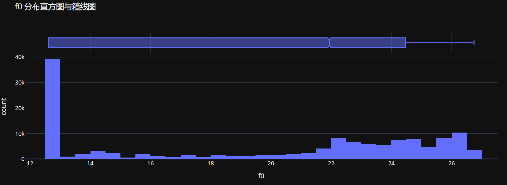
# 3.1 分布直方图
for i, feature in enumerate(numeric_features[:1]): # 只分析前1个特征
fig = px.histogram(df, x=feature, marginal="box",
title=f'{feature} 分布直方图与箱线图',
nbins=50)
fig.show()
# 3.2 统计摘要表
feature_stats = []
for feature in numeric_features:
stats_data = {
'Feature': feature,
'Mean': df[feature].mean(),
'Median': df[feature].median(),
'Std': df[feature].std(),
'Min': df[feature].min(),
'Max': df[feature].max(),
'Skewness': df[feature].skew(),
'Kurtosis': df[feature].kurtosis(),
'Missing': df[feature].isnull().sum()
}
feature_stats.append(stats_data)
feature_stats_df = pd.DataFrame(feature_stats)
print("数值特征统计摘要:")
print(feature_stats_df)
# 3.3 异常值检测
outlier_stats = []
for feature in numeric_features:
Q1 = df[feature].quantile(0.25)
Q3 = df[feature].quantile(0.75)
IQR = Q3 - Q1
lower_bound = Q1 - 1.5 * IQR
upper_bound = Q3 + 1.5 * IQR
outliers = df[(df[feature] < lower_bound) | (df[feature] > upper_bound)].shape[0]
outlier_percentage = (outliers / len(df)) * 100
outlier_stats.append({
'Feature': feature,
'Outliers': outliers,
'Outlier_Percentage': outlier_percentage,
'Lower_Bound': lower_bound,
'Upper_Bound': upper_bound
})
outlier_stats_df = pd.DataFrame(outlier_stats)
print("\n异常值统计:")
print(outlier_stats_df)
# 4. 特征与目标变量关系分析
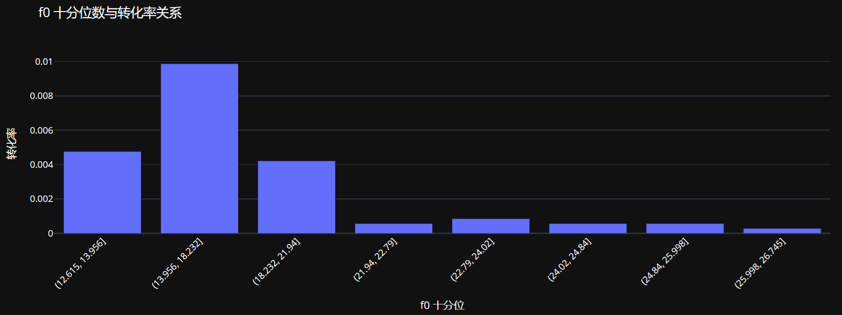
# 4.1 数值特征与转化率的关系
for feature in numeric_features[:1]: # 只分析前1个特征
# 创建十分位数分箱
df['decile'] = pd.qcut(df[feature], q=10, duplicates='drop')
# 将 Interval 对象转换为字符串
df['decile_str'] = df['decile'].astype(str)
decile_ctr = df.groupby('decile_str')['conversion'].mean().reset_index()
fig = px.bar(decile_ctr, x='decile_str', y='conversion',
title=f'{feature} 十分位数与转化率关系',
labels={'decile_str': f'{feature} 十分位', 'conversion': '转化率'})
fig.update_layout(xaxis_tickangle=-45)
fig.show()
# 散点图(采样以避免过度绘制)
sample_df = df.sample(n=min(5000, len(df)), random_state=42)
fig = px.scatter(sample_df, x=feature, y='conversion',
trendline="lowess",
title=f'{feature} 与转化率关系散点图',
opacity=0.5)
fig.show()
# 4.2 特征与处理组交互效应
for feature in numeric_features[:1]:
    # 处理组和对照组的特征分布对比
    fig = px.box(df, x='treatment', y=feature,
                 title=f'{feature} 在处理组和对照组中的分布')
    fig.show()

    # 计算处理组和对照组中特征与转化的相关性差异
    treatment_corr = df[df['treatment'] == 1][[feature, 'conversion']].corr().iloc[0, 1]
    control_corr = df[df['treatment'] == 0][[feature, 'conversion']].corr().iloc[0, 1]

    print(f"{feature} 与转化的相关性 - 处理组: {treatment_corr:.3f}, 对照组: {control_corr:.3f}")
# 5. 多变量分析
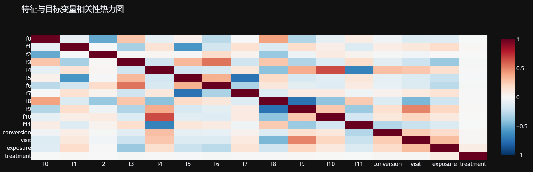
# 5.1 相关性矩阵
corr_matrix = df[numeric_features + target_variables + [treatment_var]].corr()
fig = px.imshow(corr_matrix,
title='特征与目标变量相关性热力图',
aspect="auto",
color_continuous_scale='RdBu_r',
zmin=-1, zmax=1)
fig.show()
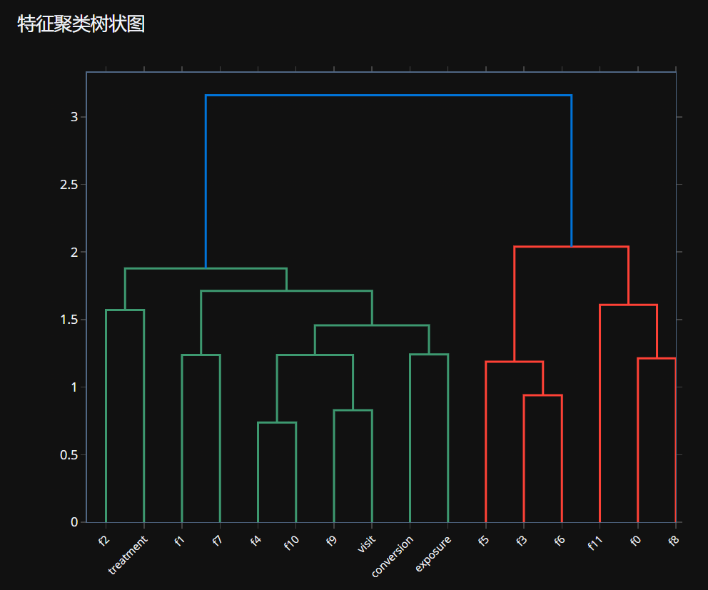
# 5.2.1 特征聚类树状图
# 创建树状图
dendro = ff.create_dendrogram(corr_matrix,
                             orientation='bottom',
                             labels=corr_matrix.columns.tolist())  # 明确设置标签

# 更新树状图布局
dendro.update_layout(
    height=600,
    title_text="特征聚类树状图",
    showlegend=False,
    margin=dict(l=100, r=50, t=80, b=100)
)

# 调整x轴标签 - 旋转并确保显示
dendro.update_xaxes(
    tickangle=-45,      # 旋转标签避免重叠
    tickfont=dict(size=10)  # 调整字体大小
)

# 显示树状图
dendro.show()
# 5.2.2 特征相关性热力图(下方图片)
# 创建热力图
heatmap = go.Heatmap(z=corr_matrix.values,
                     x=corr_matrix.columns,
                     y=corr_matrix.index,
                     colorscale='RdBu_r',
                     zmin=-1, zmax=1)

# 创建独立的热力图图表
fig_heatmap = go.Figure(data=[heatmap])

# 更新热力图布局
fig_heatmap.update_layout(
    title_text="特征相关性热力图",
    margin=dict(l=100, r=50, t=80, b=100)
)

# 反转热力图的y轴以匹配树状图的顺序
fig_heatmap.update_yaxes(autorange="reversed")

# 显示热力图
fig_heatmap.show()
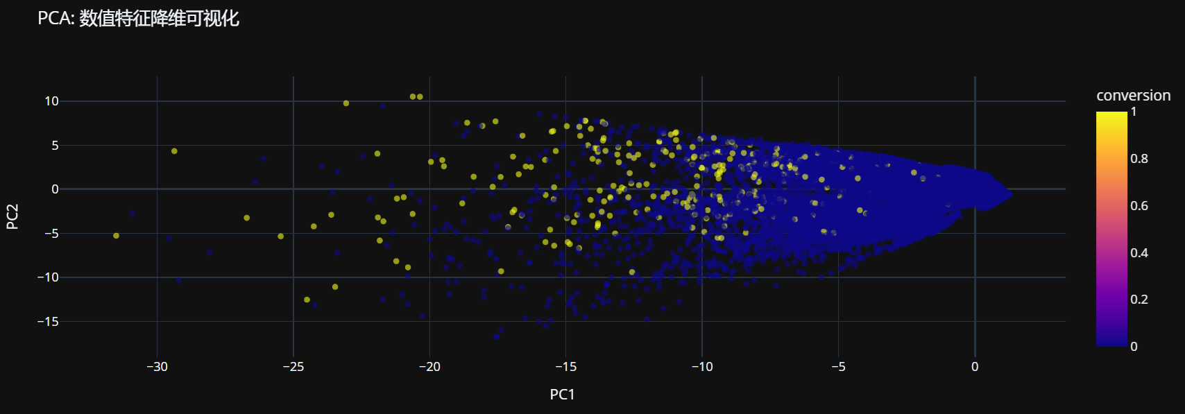
# 5.3 主成分分析 (PCA) 可视化
from sklearn.decomposition import PCA
from sklearn.preprocessing import StandardScaler

# 选择数值特征进行PCA
X = df[numeric_features].fillna(df[numeric_features].median())

# 标准化数据
scaler = StandardScaler()
X_scaled = scaler.fit_transform(X)

# 应用PCA
pca = PCA(n_components=2)
principal_components = pca.fit_transform(X_scaled)

# 创建PCA结果 DataFrame
pca_df = pd.DataFrame(data=principal_components,
                      columns=['PC1', 'PC2'])
pca_df['conversion'] = df['conversion'].values
pca_df['treatment'] = df['treatment'].values

# 可视化PCA结果
fig = px.scatter(pca_df, x='PC1', y='PC2', color='conversion',
                 title='PCA: 数值特征降维可视化',
                 opacity=0.6)
fig.show()
# 6. 特征重要性分析
# 6.1 基于随机森林的特征重要性
from sklearn.ensemble import RandomForestClassifier
from sklearn.model_selection import train_test_split

# 准备数据
X = df[numeric_features].fillna(df[numeric_features].median())
y = df['conversion']

# 划分训练测试集
X_train, X_test, y_train, y_test = train_test_split(X, y, test_size=0.3, random_state=42)

# 训练随机森林模型
rf = RandomForestClassifier(n_estimators=100, random_state=42)
rf.fit(X_train, y_train)

# 获取特征重要性
feature_importance = pd.DataFrame({
    'feature': numeric_features,
    'importance': rf.feature_importances_
}).sort_values('importance', ascending=False)

# 可视化特征重要性
fig = px.bar(feature_importance, x='importance', y='feature', orientation='h',
             title='基于随机森林的特征重要性排序',
             labels={'importance': '重要性', 'feature': '特征'})
fig.show()
# 6.2 基于互信息的特征重要性
from sklearn.feature_selection import mutual_info_classif

# 计算互信息
mi_scores = mutual_info_classif(X, y, random_state=42)
mi_df = pd.DataFrame({
    'feature': numeric_features,
    'mi_score': mi_scores
}).sort_values('mi_score', ascending=False)

# 可视化互信息得分
fig = px.bar(mi_df, x='mi_score', y='feature', orientation='h',
             title='基于互信息的特征重要性排序',
             labels={'mi_score': '互信息得分', 'feature': '特征'})
fig.show()
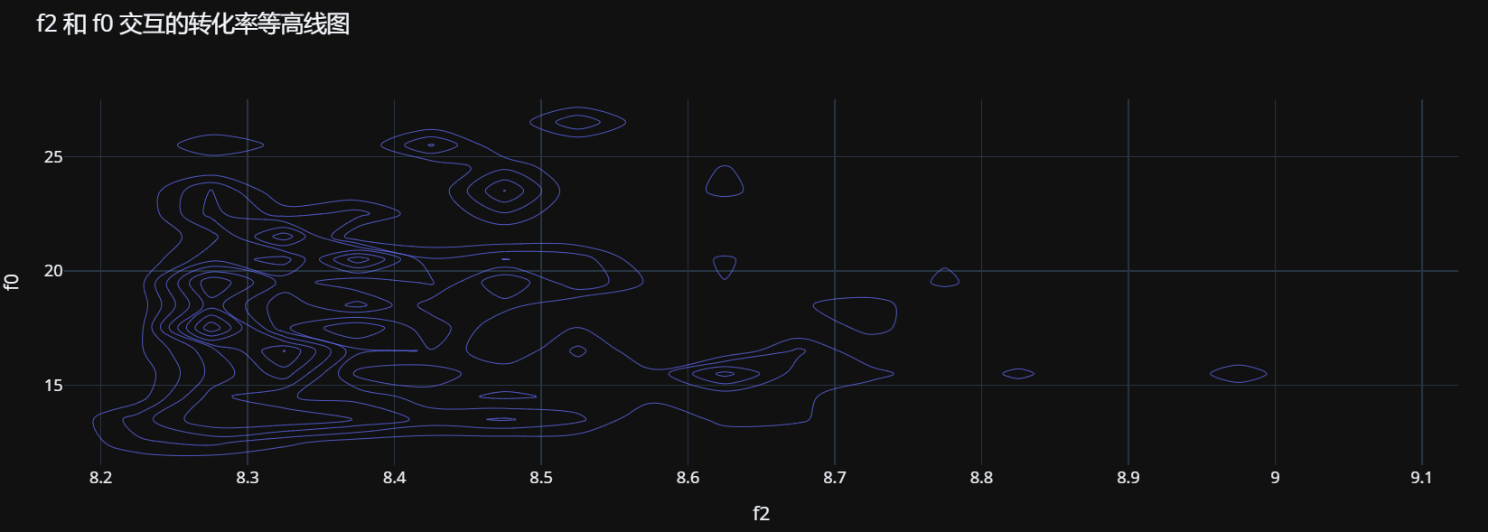
# 7. 特征交互效应分析
# 7.1 选择两个最重要的特征分析交互效应
top_features = feature_importance.head(2)['feature'].values

if len(top_features) == 2:
    feature1, feature2 = top_features

    # 创建3D散点图
    sample_df = df.sample(n=min(3000, len(df)), random_state=42)
    fig = px.scatter_3d(sample_df, x=feature1, y=feature2, z='conversion',
                        color='conversion', opacity=0.7,
                        title=f'{feature1} 和 {feature2} 与转化率的交互效应')
    fig.show()

    # 创建二维等高线图
    fig = px.density_contour(df, x=feature1, y=feature2, z='conversion',
                             histfunc='avg',
                             title=f'{feature1} 和 {feature2} 交互的转化率等高线图')
    fig.show()
# 9. 高级特征洞察
# 9.1 特征分布对比:转化用户 vs 非转化用户
for feature in numeric_features[:1]:
    converted = df[df['conversion'] == 1][feature]
    not_converted = df[df['conversion'] == 0][feature]

    # 创建分布对比图
    fig = ff.create_distplot([converted, not_converted],
                             ['转化用户', '非转化用户'],
                             bin_size=0.2, show_rug=False)
    fig.update_layout(title_text=f'{feature} 在转化与非转化用户中的分布对比')
    fig.show()

    # 执行t检验
    t_stat, p_value = stats.ttest_ind(converted, not_converted, nan_policy='omit')
    print(f"{feature} 的t检验: t={t_stat:.3f}, p={p_value:.3f}")
# 9.2 特征工程建议
print("\n特征工程建议:")
for feature in numeric_features:
    skewness = df[feature].skew()
    if abs(skewness) > 1:
        print(f"- {feature} 偏度较高 ({skewness:.2f}),考虑进行对数变换或Box-Cox变换")

    # 检查特征是否具有大量零值
    zero_percentage = (df[feature] == 0).sum() / len(df) * 100
    if zero_percentage > 50:
        print(f"- {feature} 有 {zero_percentage:.1f}% 的零值,考虑创建二元标志特征")
# 10. 保存分析结果
feature_stats_df.to_csv('feature_statistics.csv', index=False)
outlier_stats_df.to_csv('outlier_statistics.csv', index=False)
feature_importance.to_csv('feature_importance.csv', index=False)

print("特征探索完成! 详细统计结果已保存到CSV文件。")

# 创建2x2的子图布局
fig = make_subplots(
    rows=2, cols=2,
    subplot_titles=('Treatment Distribution (1=Group)',
                   'Exposure Distribution (1=Exposed)',
                   'Conversion Distribution (1=Converted)',
                   'Visit Distribution (1=Visited)')
)

# 计算每个变量的计数
treatment_counts = df['treatment'].value_counts().sort_index()
exposure_counts = df['exposure'].value_counts().sort_index()
conversion_counts = df['conversion'].value_counts().sort_index()
visit_counts = df['visit'].value_counts().sort_index()

# 添加treatment分布图
fig.add_trace(
    go.Bar(x=treatment_counts.index, y=treatment_counts.values,
           name="Treatment", marker_color=px.colors.qualitative.Set1[0]),
    row=1, col=1
)

# 添加exposure分布图
fig.add_trace(
    go.Bar(x=exposure_counts.index, y=exposure_counts.values,
           name="Exposure", marker_color=px.colors.qualitative.Set1[1]),
    row=1, col=2
)

# 添加conversion分布图
fig.add_trace(
    go.Bar(x=conversion_counts.index, y=conversion_counts.values,
           name="Conversion", marker_color=px.colors.qualitative.Set1[2]),
    row=2, col=1
)

# 添加visit分布图
fig.add_trace(
    go.Bar(x=visit_counts.index, y=visit_counts.values,
           name="Visit", marker_color=px.colors.qualitative.Set1[3]),
    row=2, col=2
)

# 更新布局
fig.update_layout(
    title_text="关键变量分布分析",
    height=600,
    showlegend=False,
    template="plotly_white"  # 使用白色网格背景,类似于seaborn的whitegrid
)

# 更新x轴和y轴标签
fig.update_xaxes(title_text="Value", row=1, col=1)
fig.update_xaxes(title_text="Value", row=1, col=2)
fig.update_xaxes(title_text="Value", row=2, col=1)
fig.update_xaxes(title_text="Value", row=2, col=2)

fig.update_yaxes(title_text="Count", row=1, col=1)
fig.update_yaxes(title_text="Count", row=1, col=2)
fig.update_yaxes(title_text="Count", row=2, col=1)
fig.update_yaxes(title_text="Count", row=2, col=2)

# 显示图形
fig.show()

# 打印具体比例
print(f"Treatment Group 比例: {df['treatment'].mean():.4f}")
print(f"实际曝光率 (Exposure): {df['exposure'].mean():.4f}")
print(f"整体转化率 (Conversion): {df['conversion'].mean():.4f}")
print(f"整体访问率 (Visit): {df['visit'].mean():.4f}")

Treatment Group 比例: 0.8494
- 实际曝光率 (Exposure): 0.0310
- 整体转化率 (Conversion): 0.0031
- 整体访问率 (Visit): 0.0473
初步ITT估计
进行初步ITT(Intention-To-Treat)分析是因果推断中至关重要的一步,其核心目的可以概括为:评估“策略或干预措施本身”的“真实世界”整体有效性,而不是在理想条件下该策略的“理论”有效性。它是一种从“上帝视角”或“决策者视角”进行的评估。
核心目的:估计“策略部署”的净效果
想象一下,公司决定对一部分用户投放一个新广告(处理组),另一部分不投放(对照组)。ITT分析回答的问题是:“决定给用户投放这个广告,最终为我们带来了多少额外的转化?”它衡量的是处理分配(Intention) 本身带来的宏观平均效果,而不是处理接收(Treatment Received)的效果。
为什么ITT估计如此重要和实用?
- 反映现实世界的真实影响。在现实世界中,任何策略的执行都不可能完美:
- 处理组中:有些用户可能根本没看到广告(广告位没加载、用户快速划走)。
- 对照组中:有些用户可能通过其他渠道接触到了类似广告。
- ITT包含了所有这些“不完美”的情况。它告诉你,当你决定实施这个策略时,最终能期望得到什么样的整体业务提升。这对于高层决策者(如CEO、产品总监)至关重要,因为他们关心的是战略层面的投入产出比(ROI)。
- 避免“选择偏差”。如果我们只分析那些“真正看到广告的用户”和“没看到广告的用户”,就会引入巨大的偏差。因为“看到广告”这个行为本身就不是随机的——可能是更活跃的用户、更爱点击的用户才看到了广告。比较这两个群体,得出的效果会严重高估,因为用户本身的差异(活跃度)影响了结果。ITT通过严格遵守随机分组的原始分配,完美地保持了处理组和对照组之间的可比性,从而获得无偏的因果效应估计。
- 政策评估的黄金标准。在医学临床试验、经济学、社会科学和政策评估中,ITT被视为黄金标准。因为它回答了:“推出这项新政策/新药物,预计能对社会/病患群体产生多大的平均效益?”这比“在完美服药条件下药效有多好”这个问题的答案,对于公共卫生决策者来说更有价值。
ITT的局限性及后续步骤
虽然ITT目的明确且非常重要,但它也有其局限性:
- 效果“稀释”:由于处理组中有人没接受处理,对照组中有人意外接受了处理,ITT估计值通常会是真实处理效应的一个“稀释”后的版本(即绝对值更小)。它衡量的是策略执行的有效性,而不是策略本身的理论最大有效性。
- 无法回答异质性性问题:ITT给出的是一个平均效果。它无法告诉我们“广告对哪类用户最有效?”这类问题。
import pandas as pd
import numpy as np
import plotly.express as px
from statsmodels.formula.api import ols
import warnings
warnings.filterwarnings('ignore')

# 加载数据(这里假设已经下载了Criteo数据集)
df = pd.read_csv("data/criteo-data.csv")

numeric_features = [f'f{i}' for i in range(12)]

# 初步ITT分析
# 计算处理组和对照组的转化率
conversion_rates = df.groupby('treatment')['conversion'].agg(['mean', 'count', 'std'])
conversion_rates.columns = ['conversion_rate', 'count', 'std']

print("\n处理组和对照组的转化率:")
print(conversion_rates)

# 计算ITT估计值
treatment_conversion = conversion_rates.loc[1, 'conversion_rate']
control_conversion = conversion_rates.loc[0, 'conversion_rate']
itt_estimate = treatment_conversion - control_conversion

print(f"\nITT估计值: {itt_estimate:.6f}")

# 统计显著性检验
# 使用t检验评估ITT的统计显著性
from scipy import stats

treatment_group = df[df['treatment'] == 1]['conversion']
control_group = df[df['treatment'] == 0]['conversion']

t_stat, p_value = stats.ttest_ind(treatment_group, control_group, equal_var=False)

print(f"t统计量: {t_stat:.4f}")
print(f"p值: {p_value:.6f}")

# 计算置信区间
def calculate_ci(mean1, mean2, std1, std2, n1, n2, alpha=0.95):
    """计算两组均值差异的置信区间"""
    mean_diff = mean1 - mean2
    std_err = np.sqrt((std1**2 / n1) + (std2**2 / n2))
    margin_error = stats.t.ppf((1 + alpha) / 2, min(n1, n2) - 1) * std_err
    ci_lower = mean_diff - margin_error
    ci_upper = mean_diff + margin_error
    return ci_lower, ci_upper

ci_lower, ci_upper = calculate_ci(
    treatment_conversion, control_conversion,
    conversion_rates.loc[1, 'std'], conversion_rates.loc[0, 'std'],
    conversion_rates.loc[1, 'count'], conversion_rates.loc[0, 'count']
)

print(f"95%置信区间: [{ci_lower:.6f}, {ci_upper:.6f}]")

# 可视化ITT结果
# 创建处理组和对照组转化率的柱状图
fig = px.bar(x=['处理组', '对照组'],
             y=[treatment_conversion, control_conversion],
             title='处理组和对照组的转化率比较',
             labels={'x': '组别', 'y': '转化率'},
             text=[f'{treatment_conversion:.4f}', f'{control_conversion:.4f}'])
fig.update_traces(texttemplate='%{text:.4f}', textposition='outside')
fig.add_annotation(x=0.5, y=max(treatment_conversion, control_conversion) + 0.01,
                   text=f"ITT估计值: {itt_estimate:.6f}<br>p值: {p_value:.6f}",
                   showarrow=False)
fig.show()

# 按特征分组的ITT分析
# 选择几个重要特征进行分析(这里假设f0-f3是重要特征)
features_to_analyze = ['f0', 'f1', 'f2', 'f3']

for feature in features_to_analyze:
    # 将连续特征分箱
    if df[feature].nunique() > 10:
        # 使用标签而不是Interval对象
        df[f'{feature}_bin'] = pd.qcut(df[feature], q=5, duplicates='drop', labels=False)
        group_var = f'{feature}_bin'

        # 为每个分箱创建有意义的标签
        bins = pd.qcut(df[feature], q=5, duplicates='drop')
        bin_labels = [f'分箱 {i+1}: {bins.cat.categories[i]}' for i in range(len(bins.cat.categories))]

        # 将数值标签映射为有意义的字符串标签
        df[f'{feature}_bin_str'] = df[group_var].map(lambda x: bin_labels[x] if not pd.isna(x) else '缺失值')
        group_var = f'{feature}_bin_str'
    else:
        # 对于类别特征,直接使用原始值
        group_var = feature
        df[group_var] = df[group_var].astype(str)

    # 计算每个分组的ITT
    grouped_itt = df.groupby(group_var).apply(
        lambda x: pd.Series({
            'treatment_rate': x['treatment'].mean(),
            'conversion_rate': x['conversion'].mean(),
            'itt_estimate': x[x['treatment'] == 1]['conversion'].mean() -
                           x[x['treatment'] == 0]['conversion'].mean(),
            'count': len(x)
        })
    ).reset_index()

    # 可视化按特征分组的ITT
    fig = px.bar(grouped_itt, x=group_var, y='itt_estimate',
                 title=f'按 {feature} 分组的ITT估计',
                 labels={group_var: feature, 'itt_estimate': 'ITT估计值'})
    fig.add_hline(y=itt_estimate, line_dash="dash", line_color="red",
                 annotation_text="总体ITT")
    fig.update_layout(xaxis_tickangle=-45)
    fig.show()

# 6. 使用线性回归进行ITT估计(考虑协变量)
# 这种方法可以控制其他变量的影响,得到更精确的ITT估计
formula = 'conversion ~ treatment + ' + ' + '.join(numeric_features)
model = ols(formula, data=df).fit()
print("\n线性回归结果 (控制协变量):")
print(model.summary())

# 提取处理效应的估计值和置信区间
treatment_effect = model.params['treatment']
treatment_ci_lower = model.conf_int().loc['treatment', 0]
treatment_ci_upper = model.conf_int().loc['treatment', 1]

print(f"\n控制协变量后的处理效应: {treatment_effect:.6f}")
print(f"95%置信区间: [{treatment_ci_lower:.6f}, {treatment_ci_upper:.6f}]")

# 7. 异质性处理效应探索
# 检查处理效应是否在不同特征水平上存在差异
interaction_results = []
for feature in features_to_analyze:
    formula = f'conversion ~ treatment * {feature}'
    model = ols(formula, data=df).fit()
    interaction_effect = model.params[f'treatment:{feature}']
    interaction_pvalue = model.pvalues[f'treatment:{feature}']
    interaction_results.append({
        'feature': feature,
        'interaction_effect': interaction_effect,
        'p_value': interaction_pvalue
    })

interaction_df = pd.DataFrame(interaction_results)
print("\n处理效应异质性分析 (交互项):")
print(interaction_df)

# 可视化交互效应
fig = px.bar(interaction_df, x='feature', y='interaction_effect',
             title='处理效应的异质性分析',
             labels={'feature': '特征', 'interaction_effect': '交互效应'},
             color='p_value',
             color_continuous_scale='viridis_r')
fig.add_hline(y=0, line_dash="dash", line_color="red")
fig.show()

# 8. 敏感性分析
# 检查ITT估计对模型设定的敏感性
# 使用不同的模型设定重新估计ITT
models = {
    '简单均值差异': itt_estimate,
    '控制所有协变量': treatment_effect,
}

# 添加只控制部分协变量的模型
for feature in features_to_analyze[:2]:
    formula = f'conversion ~ treatment + {feature}'
    model = ols(formula, data=df).fit()
    models[f'控制{feature}'] = model.params['treatment']

# 可视化不同模型的ITT估计
sensitivity_df = pd.DataFrame.from_dict(models, orient='index', columns=['ITT估计']).reset_index()
sensitivity_df.columns = ['模型', 'ITT估计']

fig = px.bar(sensitivity_df, x='模型', y='ITT估计',
             title='ITT估计的敏感性分析',
             labels={'模型': '模型设定', 'ITT估计': 'ITT估计值'})
fig.update_layout(xaxis_tickangle=-45)
fig.show()

# 9. 报告主要发现
print("\n" + "="*50)
print("ITT估计主要发现:")
print("="*50)
print(f"1. 初步ITT估计值: {itt_estimate:.6f}")
print(f"2. 统计显著性: {'显著' if p_value < 0.05 else '不显著'} (p值: {p_value:.6f})")
print(f"3. 95%置信区间: [{ci_lower:.6f}, {ci_upper:.6f}]")
print(f"4. 控制协变量后的ITT估计: {treatment_effect:.6f}")
print(f"5. 处理效应可能存在的异质性: {len(interaction_df[interaction_df['p_value'] < 0.05])} 个特征显示显著交互效应")

# 计算提升百分比
if control_conversion > 0:
    lift_percentage = (itt_estimate / control_conversion) * 100
    print(f"6. 相对于对照组的提升: {lift_percentage:.2f}%")
else:
    print("6. 对照组转化率为零,无法计算提升百分比")

print("="*50)

# 10. 保存结果到文件
results = {
    'itt_estimate': itt_estimate,
    'p_value': p_value,
    'ci_lower': ci_lower,
    'ci_upper': ci_upper,
    'treatment_effect_with_covariates': treatment_effect,
    'treatment_ci_lower': treatment_ci_lower,
    'treatment_ci_upper': treatment_ci_upper
}

results_df = pd.DataFrame.from_dict(results, orient='index', columns=['值'])
results_df.to_csv('itt_estimation_results.csv')
print("结果已保存到 itt_estimation_results.csv")
处理组和对照组的转化率:
           conversion_rate   count       std
treatment
0                 0.001615   21048  0.040160
1                 0.003394  118748  0.058157

ITT估计值: 0.001778
t统计量: 5.4854
p值: 0.000000
95%置信区间: [0.001143, 0.002414]
线性回归结果 (控制协变量):
                            OLS Regression Results
==============================================================================
Dep. Variable:             conversion   R-squared:                       0.116
Model:                            OLS   Adj. R-squared:                  0.115
Method:                 Least Squares   F-statistic:                     1405.
Date:                Thu, 16 Oct 2025   Prob (F-statistic):               0.00
Time:                        10:23:23   Log-Likelihood:             2.1361e+05
No. Observations:              139796   AIC:                        -4.272e+05
Df Residuals:                  139782   BIC:                        -4.271e+05
Df Model:                          13
Covariance Type:            nonrobust
==============================================================================
                 coef    std err          t      P>|t|      [0.025      0.975]
------------------------------------------------------------------------------
Intercept     -0.1903      0.035     -5.438      0.000      -0.259      -0.122
treatment      0.0013      0.000      3.421      0.001       0.001       0.002
f0         -8.136e-05   3.92e-05     -2.073      0.038      -0.000   -4.45e-06
f1            -0.0079      0.002     -4.007      0.000      -0.012      -0.004
f2            -0.0017      0.001     -2.439      0.015      -0.003      -0.000
f3            -0.0011      0.000     -7.172      0.000      -0.001      -0.001
f4             0.0464      0.001     55.121      0.000       0.045       0.048
f5            -0.0054      0.001     -7.499      0.000      -0.007      -0.004
f6            -0.0002   4.57e-05     -5.122      0.000      -0.000      -0.000
f7            -0.0010      0.000     -4.617      0.000      -0.001      -0.001
f8            -0.0019      0.005     -0.363      0.717      -0.012       0.008
f9             0.0002   3.92e-05      6.092      0.000       0.000       0.000
f10           -0.0376      0.001    -29.058      0.000      -0.040      -0.035
f11           -0.2551      0.010    -25.779      0.000      -0.274      -0.236
==============================================================================
Omnibus:                   268075.996   Durbin-Watson:                   2.003
Prob(Omnibus):                  0.000   Jarque-Bera (JB):        441942011.489
Skew:                          15.249   Prob(JB):                         0.00
Kurtosis:                     276.755   Cond. No.                     8.19e+03
==============================================================================

Notes:
[1] Standard Errors assume that the covariance matrix of the errors is correctly specified.
[2] The condition number is large, 8.19e+03. This might indicate that there are
strong multicollinearity or other numerical problems.

控制协变量后的处理效应: 0.001343
95%置信区间: [0.000574, 0.002113]

处理效应异质性分析 (交互项):
  feature  interaction_effect       p_value
0      f0           -0.000234  2.582618e-03
1      f1            0.026944  1.645609e-09
2      f2           -0.001037  4.564514e-01
3      f3           -0.002834  2.522617e-17
==================================================
ITT估计主要发现:
==================================================
1. 初步ITT估计值: 0.001778
2. 统计显著性: 显著 (p值: 0.000000)
3. 95%置信区间: [0.001143, 0.002414]
4. 控制协变量后的ITT估计: 0.001343
5. 处理效应可能存在的异质性: 3 个特征显示显著交互效应
6. 相对于对照组的提升: 110.09%
==================================================
结果已保存到 itt_estimation_results.csv
“非遵从”分析
什么是“非遵从”现象?
核心定义:在随机实验或准实验中,个体被分配到一个处理组或对照组,但并未完全遵循分配方案,导致其实际接受的处理状态与初始分配不一致。
典型场景:
- 广告实验:用户被分配到“看广告”的处理组,但因未打开App、广告加载失败等原因,并未实际曝光广告。
- 优惠券实验:用户被分配到“发送优惠券”组,但可能因未查看邮件/短信而未使用优惠券。
关键变量:
- treatment(处理分配):随机分配的组别(0=对照组,1=处理组)。这是工具变量。
- exposure(实际曝光):个体实际接受的处理状态(0=未曝光,1=曝光)。这是内生处理变量。
- conversion(转化):我们关心的结果变量(如购买、点击)。
为什么要分析“非遵从”?其危害是什么?
忽略“非遵从”会导致严重的因果推断错误:
- 选择偏差:实际曝光广告的用户(exposure=1)可能本身就是更活跃、转化意愿更高的用户。直接比较 exposure=1和 exposure=0的人群的转化率,会混淆“广告效应”和“用户自身特性”,高估广告效果。
- 低估策略效果:单纯比较处理组和对照组(Intent-To-Treat, ITT分析)衡量的是“分配策略”的整体效果。如果非遵从率很高(如4%的用户未曝光),ITT效应会严重稀释“广告曝光”的真实因果效应。
分析的根本目的:得到对处理(如广告曝光)的无偏的因果效应估计。
如何诊断“非遵从”?—— 关键诊断步骤
首先必须量化非遵从的严重程度。
import pandas as pd
import numpy as np

# 1. 创建交叉表,查看 treatment 和 exposure 的一致性
cross_tab = pd.crosstab(data['treatment'], data['exposure'], margins=True)
cross_tab_perc = pd.crosstab(data['treatment'], data['exposure'], normalize='index') # 按行计算百分比

print("Treatment vs Exposure 交叉表(计数):")
print(cross_tab)
print("\nTreatment vs Exposure 交叉表(行比例):")
print(np.round(cross_tab_perc * 100, 2))

# 2. 计算关键的非遵从比例
# - 处理组中未曝光的人 (令人遗憾的非遵从)
treatment_group_no_exposure = cross_tab.loc[1, 0] / cross_tab.loc[1, 'All']
# - 对照组中曝光的人 (令人讨厌的非遵从)
control_group_with_exposure = cross_tab.loc[0, 1] / cross_tab.loc[0, 'All']

print(f"\n关键非遵从比例:")
print(f"- 在处理组中,有 {treatment_group_no_exposure*100:.2f}% 的人未能成功曝光广告。")
print(f"- 在对照组中,有 {control_group_with_exposure*100:.2f}% 的人意外曝光了广告。")
Treatment vs Exposure 交叉表(计数):
exposure        0     1     All
treatment
0           21048     0   21048
1          114411  4337  118748
All        135459  4337  139796

Treatment vs Exposure 交叉表(行比例):
exposure        0     1
treatment
0          100.00  0.00
1           96.35  3.65
关键非遵从比例:
- 在处理组中,有 96.35% 的人未能成功曝光广告。
- 在对照组中,有 0.00% 的人意外曝光了广告。
诊断结果解读(以Criteo数据集为例):
- 对照组纯净度:对照组中00% 的人曝光广告,说明实验执行的一半是完美的。
- 处理组非遵从严重:处理组中高达40% 的人未曝光,说明广告投放的“送达率”极低。
- 实验性质转变:这不再是一个标准的A/B测试,而变成一个鼓励型设计。treatment不是一个强制命令,而是一个“机会”或“鼓励”。
如何解决“非遵从”?—— 工具变量法
当存在“非遵从”时,直接比较 exposure会导致选择偏差,而简单的 ITT分析又会稀释效应。工具变量法是解决这一难题、估计无偏因果效应的标准方法。
工具变量法的核心直觉是:寻找一个“外生的冲击”作为代理,这个冲击只通过影响我们关心的处理变量来影响结果。
一个经典的比喻:想象我们想研究“参军”对“未来收入”的影响。直接比较参军和未参军的人的收入会有偏差(因为参军的人可能来自不同社会经济背景)。但我们发现,越战时期美国使用了“征兵抽签”(Draft Lottery)号码随机决定谁被征召。这是一个绝佳的工具变量。
- 相关性:抽签号码靠前的人,参军率更高。
- 排他性约束:抽签号码本身是随机的,它不会直接影响一个人的收入能力(除了通过影响参军这个行为之外)。
于是,我们可以比较抽签号码靠前和靠后的人的收入差异,并将其归因于参军的影响。工具变量法做的就是这件事。
在案例中:
- 工具变量 (Z):treatment(随机分配)
- 内生处理变量 (D):exposure(实际曝光)
- 结果变量 (Y):conversion(转化)
工具变量必须满足两个核心假设,缺一不可:
- 相关性 (Relevance):工具变量 Z必须与内生变量 D相关。验证方法:第一阶段回归。我们运行 exposure ~ treatment的回归。
- 排他性约束 (Exclusion Restriction):工具变量 Z只能通过影响内生变量 D来影响结果 Y,不能有其他直接或间接的路径。这个假设无法被数据直接检验,必须基于逻辑和实验设计进行论证。
模型实现:两阶段最小二乘法 (2SLS)
工具变量法最常用的实现方式是两阶段最小二乘法,它直观地体现了“剥离内生性”的思想。
第一阶段 (First Stage):
用工具变量 Z(treatment) 和所有控制变量 X来回归内生变量 D(exposure)。
exposure = α + β * treatment + γ * X + ε
我们从这一步得到 exposure的预测值 exposure_hat。这个预测值只包含了由随机分配 treatment所解释的那部分变异,它已经“剥离”了与误差项相关的内生部分。
第二阶段 (Second Stage):
用第一阶段得到的、纯净的 exposure_hat去回归结果变量 Y(conversion)。
conversion = λ + δ * exposure_hat + θ * X + υ
这里的系数 δ就是我们最终想要的局部平均处理效应 (LATE) 的无偏估计。
import pandas as pd
import numpy as np
import statsmodels.api as sm
from sklearn.linear_model import LinearRegression
import plotly.graph_objects as go
from plotly.subplots import make_subplots
import plotly.express as px

# 加载数据(这里假设已经下载了Criteo数据集)
df = pd.read_csv("data/criteo-data.csv")

control_vars = ['f0', 'f1', 'f2', 'f3', 'f4', 'f5', 'f6', 'f7', 'f8', 'f9', 'f10', 'f11']
instrument_var = 'treatment'
endogenous_var = 'exposure'
outcome_var = 'conversion'


# 手动实现两阶段最小二乘法 (2SLS) - 使用Plotly可视化
print("=" * 60)
print("工具变量法 - 两阶段最小二乘法 (2SLS) 手动实现 (Plotly版本)")
print("=" * 60)

# 准备数据
X = df[control_vars]
Z = df[instrument_var]  # 工具变量
D = df[endogenous_var]  # 内生变量
Y = df[outcome_var]     # 结果变量

# 添加常数项
X_with_const = sm.add_constant(X)

# ==================== 第一阶段回归 ====================
print("\n" + "="*40)
print("第一阶段回归: 工具变量(Z) → 内生变量(D)")
print("="*40)

# 构建第一阶段回归的数据:用工具变量和控制变量预测内生变量
first_stage_data = pd.concat([Z, X], axis=1)
first_stage_data_with_const = sm.add_constant(first_stage_data)

# 第一阶段回归
first_stage_model = sm.OLS(D, first_stage_data_with_const)
first_stage_results = first_stage_model.fit()

print("第一阶段回归结果:")
print(first_stage_results.summary())

# 获取第一阶段的预测值 D_hat
D_hat = first_stage_results.fittedvalues

# 计算第一阶段的关键统计量
first_stage_f_statistic = (first_stage_results.rsquared / (1 - first_stage_results.rsquared)) * \
                         (first_stage_results.df_model / first_stage_results.df_resid)

print(f"\n第一阶段关键统计量:")
print(f"- R-squared: {first_stage_results.rsquared:.6f}")
print(f"- F统计量: {first_stage_f_statistic:.2f}")
print(f"- 工具变量系数: {first_stage_results.params[instrument_var]:.6f}")
print(f"- 工具变量系数p值: {first_stage_results.pvalues[instrument_var]:.6f}")

# 弱工具变量检验
if first_stage_f_statistic > 10:
    print("✓ 工具变量强度: 充足 (F > 10)")
else:
    print("⚠ 警告: 工具变量可能较弱 (F < 10)")
============================================================
工具变量法 - 两阶段最小二乘法 (2SLS) 手动实现 (Plotly版本)
============================================================
========================================
第一阶段回归: 工具变量(Z) → 内生变量(D)
========================================
第一阶段回归结果:
OLS Regression Results
==============================================================================
Dep. Variable: exposure R-squared: 0.174
Model: OLS Adj. R-squared: 0.174
Method: Least Squares F-statistic: 2266.
Date: Thu, 16 Oct 2025 Prob (F-statistic): 0.00
Time: 18:55:08 Log-Likelihood: 59962.
No. Observations: 139796 AIC: -1.199e+05
Df Residuals: 139782 BIC: -1.198e+05
Df Model: 13
Covariance Type: nonrobust
==============================================================================
coef std err t P>|t| [0.025 0.975]
------------------------------------------------------------------------------
const 0.5374 0.105 5.117 0.000 0.332 0.743
treatment 0.0328 0.001 27.868 0.000 0.031 0.035
f0 -0.0020 0.000 -17.033 0.000 -0.002 -0.002
f1 0.0200 0.006 3.374 0.001 0.008 0.032
f2 -0.0103 0.002 -4.830 0.000 -0.014 -0.006
f3 -0.0301 0.000 -63.745 0.000 -0.031 -0.029
f4 0.0197 0.003 7.790 0.000 0.015 0.025
f5 -0.0353 0.002 -16.298 0.000 -0.040 -0.031
f6 -0.0044 0.000 -31.826 0.000 -0.005 -0.004
f7 -0.0027 0.001 -4.314 0.000 -0.004 -0.001
f8 -0.1313 0.016 -8.377 0.000 -0.162 -0.101
f9 0.0010 0.000 8.275 0.000 0.001 0.001
f10 -0.0159 0.004 -4.095 0.000 -0.024 -0.008
f11 -0.2165 0.030 -7.289 0.000 -0.275 -0.158
==============================================================================
Omnibus: 119936.057 Durbin-Watson: 2.007
Prob(Omnibus): 0.000 Jarque-Bera (JB): 3182819.270
Skew: 4.183 Prob(JB): 0.00
Kurtosis: 24.828 Cond. No. 8.19e+03
==============================================================================
Notes:
[1] Standard Errors assume that the covariance matrix of the errors is correctly specified.
[2] The condition number is large, 8.19e+03. This might indicate that there are
strong multicollinearity or other numerical problems.
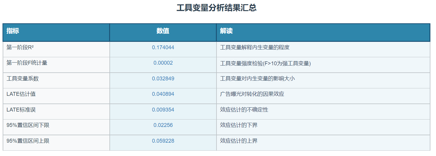
第一阶段关键统计量:
- R-squared: 0.174044
- F统计量: 0.00
- 工具变量系数: 0.032849
- 工具变量系数p值: 0.000000
⚠ 警告: 工具变量可能较弱 (F < 10)
# ==================== 第二阶段回归 ====================
print("\n" + "="*40)
print("第二阶段回归: 内生变量预测值(D_hat) → 结果变量(Y)")
print("="*40)

# 构建第二阶段回归的数据:用D_hat和控制变量预测结果变量
second_stage_data = pd.concat([pd.Series(D_hat, name='D_hat', index=X.index), X], axis=1)
second_stage_data_with_const = sm.add_constant(second_stage_data)

# 第二阶段回归
second_stage_model = sm.OLS(Y, second_stage_data_with_const)
second_stage_results = second_stage_model.fit(cov_type='HC1')  # 使用异方差稳健标准误

print("第二阶段回归结果:")
print(second_stage_results.summary())

# 获取LATE估计值
late_estimate = second_stage_results.params['D_hat']
late_se = second_stage_results.bse['D_hat']

# 计算置信区间
ci_lower = late_estimate - 1.96 * late_se
ci_upper = late_estimate + 1.96 * late_se

print(f"\n局部平均处理效应 (LATE) 估计:")
print(f"- LATE估计值: {late_estimate:.6f}")
print(f"- 标准误: {late_se:.6f}")
print(f"- 95% 置信区间: [{ci_lower:.6f}, {ci_upper:.6f}]")
print(f"- t统计量: {late_estimate/late_se:.2f}")
print(f"- p值: {second_stage_results.pvalues['D_hat']:.6f}")
========================================
第二阶段回归: 内生变量预测值(D_hat) → 结果变量(Y)
========================================
第二阶段回归结果:
                            OLS Regression Results
==============================================================================
Dep. Variable:             conversion   R-squared:                       0.116
Model:                            OLS   Adj. R-squared:                  0.115
Method:                 Least Squares   F-statistic:                     36.04
Date:                Thu, 16 Oct 2025   Prob (F-statistic):           1.02e-91
Time:                        18:56:23   Log-Likelihood:             2.1361e+05
No. Observations:              139796   AIC:                        -4.272e+05
Df Residuals:                  139782   BIC:                        -4.271e+05
Df Model:                          13
Covariance Type:                  HC1
==============================================================================
                 coef    std err          z      P>|z|      [0.025      0.975]
------------------------------------------------------------------------------
const         -0.2123      0.083     -2.545      0.011      -0.376      -0.049
D_hat          0.0409      0.009      4.372      0.000       0.023       0.059
f0          6.837e-07   4.44e-05      0.015      0.988   -8.63e-05    8.77e-05
f1            -0.0087      0.006     -1.351      0.177      -0.021       0.004
f2            -0.0013      0.001     -1.950      0.051      -0.003    6.99e-06
f3             0.0001      0.000      0.247      0.805      -0.001       0.001
f4             0.0456      0.005      8.723      0.000       0.035       0.056
f5            -0.0040      0.003     -1.564      0.118      -0.009       0.001
f6         -5.556e-05   6.61e-05     -0.841      0.400      -0.000    7.39e-05
f7            -0.0008      0.001     -1.426      0.154      -0.002       0.000
f8             0.0035      0.006      0.536      0.592      -0.009       0.016
f9             0.0002   6.78e-05      2.937      0.003    6.63e-05       0.000
f10           -0.0370      0.006     -6.426      0.000      -0.048      -0.026
f11           -0.2462      0.063     -3.912      0.000      -0.370      -0.123
==============================================================================
Omnibus:                   268075.996   Durbin-Watson:                   2.003
Prob(Omnibus):                  0.000   Jarque-Bera (JB):        441942011.489
Skew:                          15.249   Prob(JB):                         0.00
Kurtosis:                     276.755   Cond. No.                     8.37e+03
==============================================================================

Notes:
[1] Standard Errors are heteroscedasticity robust (HC1)
[2] The condition number is large, 8.37e+03. This might indicate that there are
strong multicollinearity or other numerical problems.

局部平均处理效应 (LATE) 估计:
- LATE估计值: 0.040894
- 标准误: 0.009354
- 95% 置信区间: [0.022560, 0.059228]
- t统计量: 4.37
- p值: 0.000012
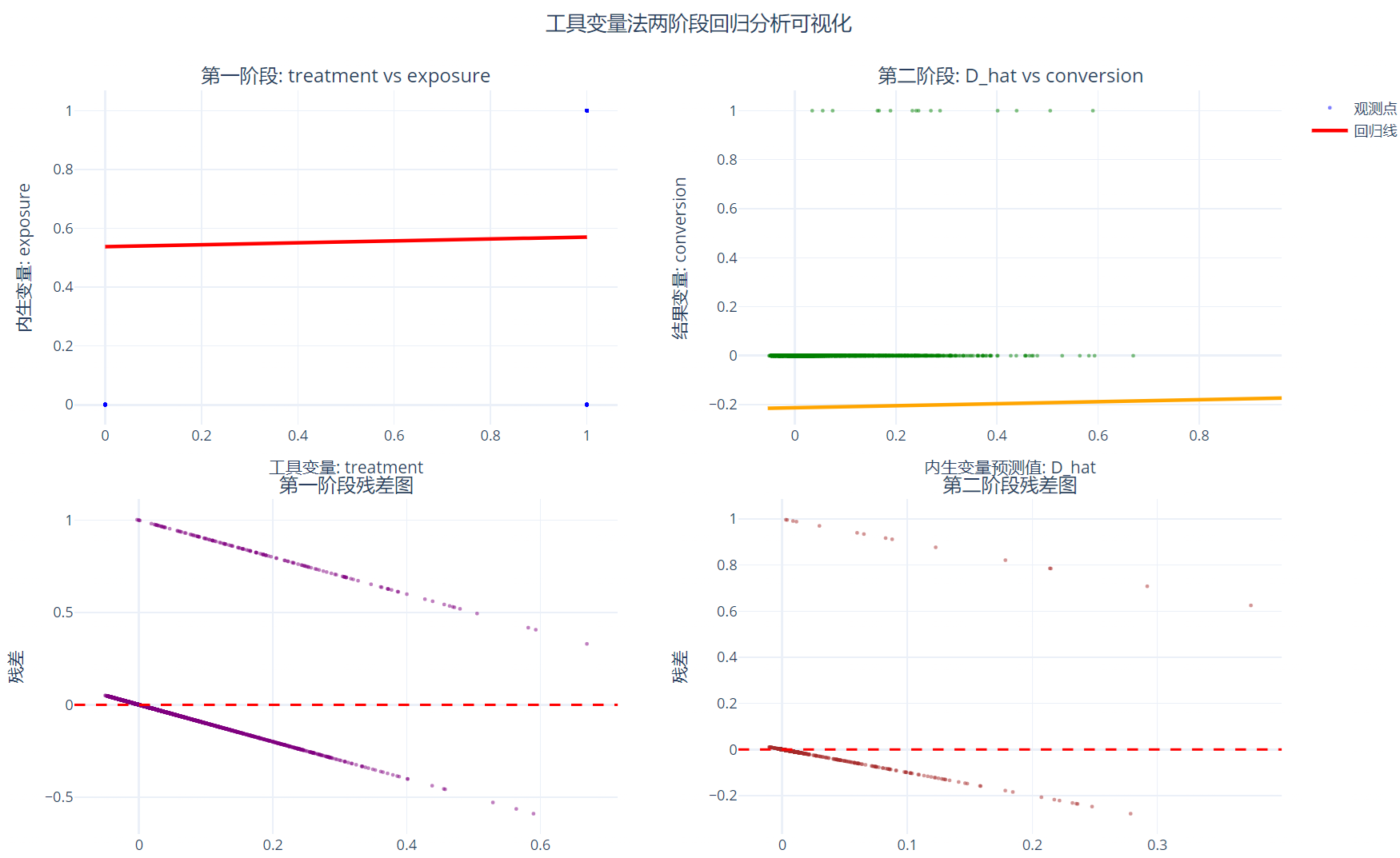
# ==================== Plotly可视化分析 ====================
print("\n" + "="*40)
print("Plotly交互式可视化分析")
print("="*40)

# 创建子图
fig = make_subplots(
    rows=2, cols=2,
    subplot_titles=[
        f'第一阶段: {instrument_var} vs {endogenous_var}',
        f'第二阶段: D_hat vs {outcome_var}',
        '第一阶段残差图',
        '第二阶段残差图'
    ],
    vertical_spacing=0.1,
    horizontal_spacing=0.1
)

# 对大样本数据进行采样以提高性能
sample_size = min(5000, len(Z))
if len(Z) > sample_size:
    sample_indices = np.random.choice(len(Z), sample_size, replace=False)
    Z_sample = Z.iloc[sample_indices]
    D_sample = D.iloc[sample_indices]
    D_hat_sample = D_hat.iloc[sample_indices]
    Y_sample = Y.iloc[sample_indices]
    first_stage_resid_sample = first_stage_results.resid.iloc[sample_indices]
    second_stage_resid_sample = second_stage_results.resid.iloc[sample_indices]
    first_stage_fitted_sample = first_stage_results.fittedvalues.iloc[sample_indices]
    second_stage_fitted_sample = second_stage_results.fittedvalues.iloc[sample_indices]
else:
    Z_sample = Z
    D_sample = D
    D_hat_sample = D_hat
    Y_sample = Y
    first_stage_resid_sample = first_stage_results.resid
    second_stage_resid_sample = second_stage_results.resid
    first_stage_fitted_sample = first_stage_results.fittedvalues
    second_stage_fitted_sample = second_stage_results.fittedvalues

# 1. 第一阶段散点图
fig.add_trace(
    go.Scatter(
        x=Z_sample, y=D_sample,
        mode='markers',
        marker=dict(size=3, opacity=0.5, color='blue'),
        name='观测点',
        hovertemplate=f'{instrument_var}: %{{x}}<br>{endogenous_var}: %{{y}}<extra></extra>'
    ),
    row=1, col=1
)

# 添加回归线
z_range = np.linspace(Z.min(), Z.max(), 100)
coef = first_stage_results.params[instrument_var]
const = first_stage_results.params['const']
regression_line = const + coef * z_range

fig.add_trace(
    go.Scatter(
        x=z_range, y=regression_line,
        mode='lines',
        line=dict(color='red', width=3),
        name='回归线',
        hovertemplate=f'{instrument_var}: %{{x}}<br>预测{endogenous_var}: %{{y:.3f}}<extra></extra>'
    ),
    row=1, col=1
)

# 2. 第二阶段散点图
fig.add_trace(
    go.Scatter(
        x=D_hat_sample, y=Y_sample,
        mode='markers',
        marker=dict(size=3, opacity=0.5, color='green'),
        name='观测点',
        hovertemplate='D_hat: %{x:.3f}<br>%{y}: %{y}<extra></extra>',
        showlegend=False
    ),
    row=1, col=2
)

# 添加回归线
d_hat_range = np.linspace(D_hat.min(), D_hat.max(), 100)
coef_2nd = second_stage_results.params['D_hat']
const_2nd = second_stage_results.params['const']
regression_line_2nd = const_2nd + coef_2nd * d_hat_range

fig.add_trace(
    go.Scatter(
        x=d_hat_range, y=regression_line_2nd,
        mode='lines',
        line=dict(color='orange', width=3),
        name='回归线',
        hovertemplate='D_hat: %{x:.3f}<br>预测%{y}: %{y:.3f}<extra></extra>',
        showlegend=False
    ),
    row=1, col=2
)

# 3. 第一阶段残差图
fig.add_trace(
    go.Scatter(
        x=first_stage_fitted_sample, y=first_stage_resid_sample,
        mode='markers',
        marker=dict(size=3, opacity=0.5, color='purple'),
        name='残差',
        hovertemplate='预测值: %{x:.3f}<br>残差: %{y:.3f}<extra></extra>',
        showlegend=False
    ),
    row=2, col=1
)

# 添加零参考线
fig.add_hline(y=0, line_dash="dash", line_color="red", row=2, col=1)

# 4. 第二阶段残差图
fig.add_trace(
    go.Scatter(
        x=second_stage_fitted_sample, y=second_stage_resid_sample,
        mode='markers',
        marker=dict(size=3, opacity=0.5, color='brown'),
        name='残差',
        hovertemplate='预测值: %{x:.3f}<br>残差: %{y:.3f}<extra></extra>',
        showlegend=False
    ),
    row=2, col=2
)

# 添加零参考线
fig.add_hline(y=0, line_dash="dash", line_color="red", row=2, col=2)

# 更新布局
fig.update_layout(
    title_text="工具变量法两阶段回归分析可视化",
    title_x=0.5,
    height=800,
    width=1200,
    showlegend=True,
    template="plotly_white"
)

# 更新坐标轴标签
fig.update_xaxes(title_text=f"工具变量: {instrument_var}", row=1, col=1)
fig.update_yaxes(title_text=f"内生变量: {endogenous_var}", row=1, col=1)
fig.update_xaxes(title_text="内生变量预测值: D_hat", row=1, col=2)
fig.update_yaxes(title_text=f"结果变量: {outcome_var}", row=1, col=2)
fig.update_xaxes(title_text="预测值", row=2, col=1)
fig.update_yaxes(title_text="残差", row=2, col=1)
fig.update_xaxes(title_text="预测值", row=2, col=2)
fig.update_yaxes(title_text="残差", row=2, col=2)

fig.show()
# ==================== 创建结果汇总仪表板 ====================

# 创建结果汇总表格
results_summary = pd.DataFrame({
    '指标': [
        '第一阶段R²', '第一阶段F统计量', '工具变量系数',
        'LATE估计值', 'LATE标准误', '95%置信区间下限', '95%置信区间上限'
    ],
    '数值': [
        first_stage_results.rsquared,
        first_stage_f_statistic,
        first_stage_results.params[instrument_var],
        late_estimate,
        late_se,
        ci_lower,
        ci_upper
    ],
    '解读': [
        '工具变量解释内生变量的程度',
        '工具变量强度检验(F>10为强工具变量)',
        '工具变量对内生变量的影响大小',
        '广告曝光对转化的因果效应',
        '效应估计的不确定性',
        '效应估计的下界',
        '效应估计的上界'
    ]
})

# 创建结果表格图
# 创建结果表格图 - 完整样式控制版本
results_table = go.Figure(data=[go.Table(
    header=dict(
        values=['<b>指标</b>', '<b>数值</b>', '<b>解读</b>'],  # 使用HTML标签加粗
        fill_color='#2E86AB',  # 更专业的蓝色
        align=['left', 'center', 'left'],  # 每列不同的对齐方式
        font=dict(
            color='white',  # 白色字体
            size=14,  # 字体大小
            family="Arial"  # 字体家族
        ),
        height=40,  # 表头高度
        line=dict(color='#1A5276', width=2)  # 边框颜色和宽度
    ),
    cells=dict(
        values=[results_summary['指标'],
               results_summary['数值'].round(6),
               results_summary['解读']],
        fill_color=[
            '#F8F9FA',  # 第一列背景色 - 浅灰色
            '#E8F4F8',  # 第二列背景色 - 更浅的蓝色
            '#F0F7FA'   # 第三列背景色 - 非常浅的蓝色
        ],
        align=['left', 'center', 'left'],  # 单元格对齐方式
        font=dict(
            color=['#2C3E50', '#2980B9', '#34495E'],  # 每列不同的字体颜色
            size=12,
            family="Arial"
        ),
        height=35,  # 单元格高度
        line=dict(color='#BDC3C7', width=1)  # 单元格边框
    )
)])

# 更新表格布局样式
results_table.update_layout(
    title=dict(
        text='<b>工具变量分析结果汇总</b>',  # 使用HTML标签
        x=0.5,  # 标题居中
        font=dict(size=18, family="Arial", color="#2C3E50")
    ),
    width=1000,  # 表格宽度
    height=400,  # 表格高度
    margin=dict(l=20, r=20, t=60, b=20),  # 边距控制
    paper_bgcolor='white',  # 背景颜色
    plot_bgcolor='white'
)

# 添加表格边框和阴影效果
results_table.update_traces(
    columnwidth=[0.25, 0.25, 0.5],  # 控制每列宽度比例
    cells=dict(
        prefix=[None, None, None],  # 前缀,如货币符号
        suffix=[None, None, None],  # 后缀,如单位
        format=[None, None, None]   # 数字格式
    )
)

results_table.show()
# ==================== 创建效应可视化图 ====================

effect_fig = go.Figure()

# 添加点估计
effect_fig.add_trace(go.Scatter(
    x=[late_estimate], y=['LATE估计'],
    mode='markers',
    marker=dict(size=15, color='blue'),
    name='点估计',
    error_x=dict(
        type='data',
        array=[late_se * 1.96],
        thickness=5,
        width=10
    )
))

# 添加置信区间
effect_fig.add_trace(go.Scatter(
    x=[ci_lower, ci_upper], y=['置信区间', '置信区间'],
    mode='lines',
    line=dict(width=10, color='gray'),
    name='95%置信区间'
))

effect_fig.update_layout(
    title='局部平均处理效应(LATE)估计',
    xaxis_title='效应大小',
    yaxis_title='',
    showlegend=True,
    width=800,
    height=400,
    template="plotly_white"
)

# 添加零线参考
effect_fig.add_vline(x=0, line_dash="dash", line_color="red")

effect_fig.show()
CausalML使用实例
特征工程
import pandas as pd
import numpy as np
from sklearn.preprocessing import StandardScaler, KBinsDiscretizer
from sklearn.model_selection import train_test_split
import category_encoders as ce

data = pd.read_csv('data/criteo-data.csv')
# 设置参数
SAMPLE_FRAC = 0.3  # 采样比例,全量数据设为1.0
N_BINS = 10  # 分箱数量
TEST_SIZE = 0.2  # 测试集比例
RANDOM_STATE = 42  # 随机种子

# 步骤: 定义特征列
numerical_cols = [f'f{i}' for i in range(12)]
treatment_col = 'treatment'
target_cols = ['conversion', 'visit', 'exposure']

# 步骤1 处理缺失值
# 数值特征:用中位数填充,如果中位数是NaN则用0填充
for col in numerical_cols:
    median_val = data[col].median()
    # 如果中位数是NaN(即整个列都是缺失值),则用0填充
    if pd.isna(median_val):
        data[col] = data[col].fillna(0)
    else:
        data[col] = data[col].fillna(median_val)

# 步骤2: 数值特征处理
# 对数变换(减少偏度) - 确保值非负
for col in numerical_cols:
    # 确保最小值大于等于0(对数变换要求)
    min_val = data[col].min()
    if min_val < 0:
        # 如果最小值小于0,将所有值平移
        data[col] = data[col] - min_val + 1e-6
    data[col] = np.log1p(data[col])

# 标准化
scaler = StandardScaler()
data[numerical_cols] = scaler.fit_transform(data[numerical_cols])

# 分箱处理(创建新特征)
binner = KBinsDiscretizer(n_bins=N_BINS, encode='ordinal', strategy='quantile')
for col in numerical_cols:
    bin_col_name = f'{col}_bin'

    # 确保列中没有NaN值
    if data[col].isna().any():
        # 如果还有NaN,用0填充
        data[col] = data[col].fillna(0)

    # 确保列中没有无穷大值
    if np.isinf(data[col]).any():
        # 用最大值替换正无穷,最小值替换负无穷
        max_val = data[col][~np.isinf(data[col])].max()
        min_val = data[col][~np.isinf(data[col])].min()
        data[col] = data[col].replace(np.inf, max_val)
        data[col] = data[col].replace(-np.inf, min_val)

    # 执行分箱
    data[bin_col_name] = binner.fit_transform(data[[col]]).astype(int)

# 步骤3: 创建增量建模专用特征
# 实验组/对照组特征差异
for col in numerical_cols:
    data[f'{col}_treat_diff'] = data[col] * data[treatment_col]
增量建模特征
data[f'{col}_treat_diff’] = data[col] * data[treatment_col]的作用
这个步骤是增量建模(Uplift Modeling)中非常关键的特征工程操作,它创建了原始特征与处理变量(treatment)的交互特征。以下是其详细作用和意义:捕捉异质性处理效应(Heterogeneous Treatment Effects)
- 核心目的:识别不同特征值的用户对处理(treatment)的不同响应
- 工作原理:通过将用户特征与处理变量相乘,创建能够反映”当用户具有特定特征值时,处理对其影响程度”的特征
- 数学表达:如果原始特征为X,处理变量为T(0或1),则新特征为X*T
为什么这在增量建模中至关重要?
在增量建模中,我们关心的不是简单的”用户是否会转化”,而是”处理(如广告)是否会导致用户转化”。这种特征交互能够:
- 区分自然转化和因果转化
- 自然转化:无论是否看到广告都会转化的用户
- 因果转化:因为看到广告才转化的用户
- 识别敏感用户群体:
- 帮助模型识别哪些特征的用户对处理最敏感(persuadable)
- 避免对不敏感用户(lost-cause或sure-thing)浪费资源
实际应用示例
假设我们有一个特征”用户活跃度”(activity_level):
- 用户A:activity_level = 0.8(高活跃用户)
- 用户B:activity_level = 0.2(低活跃用户)
创建交互特征后:
- 用户A(实验组):activity_level_treat_diff = 0.8 * 1 = 0.8
- 用户A(对照组):activity_level_treat_diff = 0.8 * 0 = 0
- 用户B(实验组):activity_level_treat_diff = 0.2 * 1 = 0.2
- 用户B(对照组):activity_level_treat_diff = 0.2 * 0 = 0
模型可以学习到:
- 高活跃用户(activity_level_treat_diff值高)对广告响应更好
- 低活跃用户(activity_level_treat_diff值低)对广告响应较差
在增量模型中的作用机制
当使用如S-Learner等增量模型时:
# S-Learner模型结构
conversion = model.predict([features, treatment_interaction_features])
- 模型可以学习特征与处理的交互效应
- 通过检查交互特征的系数/重要性,可以直接评估处理对不同特征用户的影响
与传统特征工程的区别
| 传统特征工程 | 增量建模特征工程 |
| 关注特征与目标的关系 | 关注特征与处理的交互效应 |
| 优化整体预测准确率 | 优化处理效应的估计 |
| 识别高转化用户 | 识别对处理敏感的用户 |
# 步骤4: 特征交叉
# 创建特征组合
data['f0_f1'] = data['f0'] * data['f1']
data['f2_div_f3'] = data['f2'] / (data['f3'] + 1e-6)
data['f4_f5'] = data['f4'] * data['f5']
data['f6_div_f7'] = data['f6'] / (data['f7'] + 1e-6)

# 步骤5: 创建统计特征
# 基于分箱的统计特征
for col in numerical_cols:
    bin_col = f'{col}_bin'
    # 分箱内均值
    bin_mean = data.groupby(bin_col)[col].transform('mean')
    data[f'{col}_bin_mean'] = bin_mean

    # 分箱内标准差
    bin_std = data.groupby(bin_col)[col].transform('std')
    data[f'{col}_bin_std'] = bin_std.fillna(0)

# 步骤6: 创建交互特征
# 特征与treatment的交互
for col in numerical_cols[:6]:  # 对前6个特征创建交互
    data[f'{col}_treat_interaction'] = data[col] * data[treatment_col]

# 步骤7: 多项式特征
# 二次项
for col in numerical_cols[:5]:
    data[f'{col}_squared'] = data[col] ** 2
特征处理策略
在特征工程中,选择合适的处理策略至关重要。
乘法交叉 (f0_f1, f4_f5)
作用:
- 捕捉特征间的协同效应
- 识别特征间的非线性关系
- 增强模型的表达能力
适用场景:
- 当两个特征在业务上存在关联关系时(如广告点击率 × 广告展示次数)
- 当特征可能具有乘积效应时(如用户活跃度 × 用户价值)
- 当特征分布相似且可能共同影响目标时
选择建议:
- 业务理解驱动:选择业务上存在潜在协同效应的特征对
- 相关性分析:选择相关性较高的特征对进行乘法交叉
- 特征重要性:基于初步模型的特征重要性选择重要特征进行交叉
- 领域知识:根据行业经验选择(如电商中价格 × 折扣率)
除法交叉 (f2_div_f3, f6_div_f7)
作用:
- 创建比例特征
- 捕捉特征间的相对关系
- 减少量纲影响
适用场景:
- 当特征间存在比例关系时(如点击率 = 点击/展示)
- 当需要标准化特征时(如人均消费 = 总消费/用户数)
- 当特征值范围差异大时
选择建议:
- 避免分母为零:添加小常数(如1e-6)防止除零错误
- 业务意义:选择有实际业务意义的比例组合
- 特征分布:选择分母特征分布较广的组合
- 相关性验证:计算交叉特征与目标的相关系数
分箱内均值 ({col}_bin_mean)
作用:
- 提供特征平滑表示
- 减少噪声影响
- 捕捉局部趋势
适用场景:
- 当特征分布不均匀时
- 当特征与目标关系非线性时
- 当需要减少过拟合风险时
选择建议:
- 高基数特征:优先处理取值多的特征
- 非线性关系:对与目标有非线性关系的特征使用
- 重要特征:对模型重要性高的特征添加
分箱内标准差 ({col}_bin_std)
作用:
- 衡量组内变异程度
- 捕捉特征值的稳定性
- 识别异常值模式
适用场景:
- 当特征在不同取值区间变异程度不同时
- 当需要识别异常模式时
- 在风险管理或异常检测场景
选择建议:
- 金融风控:在信用评分等场景特别有用
- 波动性特征:对波动大的特征优先使用
- 补充均值:与分箱内均值配合使用
特征与treatment交互 ({col}_treat_interaction)
- 作用:
- 捕捉处理效应的异质性
- 识别对处理敏感的用户群体
- 提升增量模型性能
- 选择建议:
- 关键特征优先:选择与业务目标最相关的特征
- 多样性覆盖:选择不同类型特征(如行为、人口统计)
- 模型反馈:基于初步模型选择重要特征
- 计算效率:限制交互特征数量(如前6个)
二次项 ({col}_squared)
作用:
- 捕捉非线性关系
- 识别U型或倒U型关系
- 增强模型表达能力
适用场景:
- 当特征与目标可能存在二次关系时
- 在存在阈值效应的情况下
- 当特征分布有偏时
选择建议:
- 偏态特征:对偏度高的特征优先使用
- 重要特征:选择模型重要性高的特征
- 业务理解:根据领域知识选择可能有非线性影响的特征
- 避免过度:限制多项式特征数量(如前5个)
因果效应特征
用户响应类型特征概述
在增量建模(Uplift Modeling)中,用户响应类型特征是最核心的因果效应特征之一。它基于用户是否接受处理(treatment)和是否转化(conversion)的组合,将用户分为四个关键群体:
Persuadable(可说服用户)
- 定义:接受处理(treatment=1)且转化(conversion=1)
- 特征含义:
- 广告/处理对这些用户产生了积极影响
- 如果没有处理,他们可能不会转化
- 业务价值:
- 营销活动的核心目标群体
- 增量效应的直接体现
- 处理策略:
- 优先投放广告
- 提供个性化优惠
- 加强用户互动
Lost-cause(无望用户)
- 定义:接受处理(treatment=1)但未转化(conversion=0)
- 特征含义:
- 广告/处理对这些用户无效
- 即使接受处理也不会转化
- 业务价值:
- 识别无效投放对象
- 避免资源浪费的关键
- 处理策略:
- 减少或停止广告投放
- 重新评估用户价值
- 考虑用户细分(如高价值但暂时不转化)
Sure-thing(必然转化用户)
- 定义:未接受处理(treatment=0)但转化(conversion=1)
- 特征含义:
- 这些用户无论如何都会转化
- 广告/处理对他们没有增量价值
- 业务价值:
- 识别忠诚用户群体
- 避免不必要的营销成本
- 处理策略:
- 减少广告投放频率
- 提供非促销性内容
- 专注于用户留存而非获取
Do-not-disturb(勿扰用户)
- 定义:未接受处理(treatment=0)且未转化(conversion=0)
- 特征含义:
- 这些用户可能对广告反感
- 处理可能产生负面效应
- 业务价值:
- 识别潜在反感用户
- 预防负面口碑传播
- 处理策略:
- 避免主动打扰
- 提供非侵入式互动
- 谨慎测试响应阈值
目标编码
目标编码(Target Encoding)是一种强大的特征工程技术,特别适用于处理分类变量。它通过使用目标变量的统计信息来编码分类特征,从而捕捉类别与目标变量之间的关系。在增量建模中,目标编码尤为重要,因为它可以帮助模型理解不同类别用户对广告处理的响应差异。
目标编码的核心思想是将分类变量的每个类别替换为该类别下目标变量的统计量(通常是均值)。例如:
- 对于用户所在城市特征:
- 城市A的用户平均转化率为15
- 城市B的用户平均转化率为08
- 编码后:
- 城市A →15
- 城市B →08
from sklearn.model_selection import KFold
# 步骤8: 创建因果效应特征 - 用户响应类型(在完整数据集上)
print("步骤8: 创建因果效应特征 - 用户响应类型...")
conditions = [
    (data['treatment'] == 1) & (data['conversion'] == 1),
    (data['treatment'] == 1) & (data['conversion'] == 0),
    (data['treatment'] == 0) & (data['conversion'] == 1),
    (data['treatment'] == 0) & (data['conversion'] == 0)
]

choices = ['persuadable', 'lost-cause', 'sure-thing', 'do-not-disturb']
data['response_type'] = np.select(conditions, choices, default='unknown')

# 步骤9: 数据集分割(包含所有特征)
print("\n步骤9: 数据集分割...")
# 为增量建模分割数据集,保持实验组/对照组比例
treatment_data = data[data['treatment'] == 1]
control_data = data[data['treatment'] == 0]

# 分割训练集和测试集
treatment_train, treatment_test = train_test_split(
    treatment_data, test_size=TEST_SIZE, random_state=RANDOM_STATE
)
control_train, control_test = train_test_split(
    control_data, test_size=TEST_SIZE, random_state=RANDOM_STATE
)

# 合并训练集和测试集(包含所有特征)
train = pd.concat([treatment_train, control_train])
test = pd.concat([treatment_test, control_test])

print(f"训练集大小: {train.shape}, 测试集大小: {test.shape}")
print(f"训练集包含特征: {train.columns.tolist()}")

# 步骤10: 目标编码处理
print("\n步骤10: 目标编码处理...")
# 定义目标编码特征 - 确保这些特征存在于分割后的数据集中
target_encode_features = [
    'f0_bin', 'f1_bin', 'f2_bin', 'f3_bin',  # 分箱特征
    'response_type',  # 用户响应类型
    'f0_f1', 'f2_div_f3'  # 交叉特征
]

# 验证特征是否存在
valid_encode_features = [f for f in target_encode_features if f in train.columns]
missing_features = set(target_encode_features) - set(valid_encode_features)

if missing_features:
    print(f"警告: 以下特征在数据集中不存在: {missing_features}")
    print("将使用可用特征进行目标编码")

# 定义目标变量
targets = ['conversion', 'visit', 'exposure']

# 创建存储编码器的字典
target_encoders = {}

# K折目标编码函数(修复版)
def kfold_target_encode(train_df, test_df, feature, target, n_folds=5):
    """
    使用K折交叉验证进行目标编码
    :param train_df: 训练集
    :param test_df: 测试集
    :param feature: 编码特征
    :param target: 目标变量
    :param n_folds: 折数
    :return: 编码后的训练集和测试集,以及编码映射
    """
    # 检查特征是否存在
    if feature not in train_df.columns:
        print(f"  错误: 特征 '{feature}' 在训练集中不存在")
        return train_df, test_df, {}

    # 创建编码列名
    new_col = f'{feature}_{target}_encoded'

    # 在训练集上计算全局均值(作为默认值)
    global_mean = train_df[target].mean()

    # 创建副本避免修改原始数据
    train_encoded = train_df.copy()
    test_encoded = test_df.copy()

    # 初始化编码列
    train_encoded[new_col] = np.nan
    test_encoded[new_col] = global_mean  # 测试集先用全局均值填充

    # K折交叉编码
    kf = KFold(n_splits=n_folds, shuffle=True, random_state=RANDOM_STATE)

    # 确保特征列存在
    if feature not in train_encoded.columns:
        print(f"  错误: 特征 '{feature}' 在训练集中不存在")
        return train_encoded, test_encoded, {}

    for train_index, val_index in kf.split(train_encoded):
        # 分割训练集和验证集
        X_train = train_encoded.iloc[train_index]
        X_val = train_encoded.iloc[val_index]

        # 计算编码值(目标均值)
        if feature in X_train.columns:
            encode_map = X_train.groupby(feature)[target].mean().to_dict()
        else:
            print(f"  错误: 特征 '{feature}' 在训练子集中不存在")
            encode_map = {}

        # 应用编码到验证集
        if feature in X_val.columns:
            val_encoded = X_val[feature].map(encode_map).fillna(global_mean)
            train_encoded.iloc[val_index, train_encoded.columns.get_loc(new_col)] = val_encoded.values

    # 计算完整训练集的编码映射(用于测试集)
    if feature in train_encoded.columns:
        full_encode_map = train_encoded.groupby(feature)[target].mean().to_dict()
        test_encoded[new_col] = test_encoded[feature].map(full_encode_map).fillna(global_mean)
    else:
        full_encode_map = {}
        test_encoded[new_col] = global_mean

    return train_encoded, test_encoded, full_encode_map

# 执行目标编码(仅使用有效特征)
for target in targets:
    print(f"\n处理目标变量: {target}")

    for feature in valid_encode_features:
        print(f"  - 编码特征: {feature}")

        # 使用K折目标编码
        train, test, encoder_map = kfold_target_encode(
            train, test, feature, target, n_folds=5
        )

        if encoder_map:  # 仅当编码成功时保存
            target_encoders[f'{feature}_{target}_kfold'] = encoder_map

# 保存编码器
import joblib
joblib.dump(target_encoders, 'target_encoders.pkl')
print("\n目标编码器已保存到 target_encoders.pkl")
增量分数特征
在增量建模中,增量分数特征(Uplift Score Feature)是最核心、最具业务价值的特征之一。它直接量化了广告处理对用户转化的因果效应,是增量建模区别于传统预测模型的关键特征。
增量分数(Uplift Score)定义为:实验组转化率 – 对照组转化率
# 步骤11: 创建增量分数特征
# 计算每个特征的增量分数
for col in numerical_cols[:5]:
    # 在训练集上计算增量分数
    treat_mean = train[train['treatment'] == 1].groupby(f'{col}_bin')['conversion'].mean()
    control_mean = train[train['treatment'] == 0].groupby(f'{col}_bin')['conversion'].mean()
    uplift_score = (treat_mean - control_mean).to_dict()

    # 应用到训练集和测试集
    train[f'{col}_uplift_score'] = train[f'{col}_bin'].map(uplift_score)
    test[f'{col}_uplift_score'] = test[f'{col}_bin'].map(uplift_score)
业务意义与价值
| 增量分数范围 | 业务解释 | 营销策略 |
| > 0.05 | 高敏感用户 | 优先投放,增加预算 |
| 0.01 – 0.05 | 中等敏感用户 | 适度投放,测试优化 |
| -0.01 – 0.01 | 低敏感用户 | 减少投放,避免打扰 |
| < -0.01 | 反感用户 | 停止投放,防止负面效应 |
# 步骤12: 特征选择(可选)
# 1. 识别并处理非数值型特征
non_numeric_cols = train.select_dtypes(exclude=['number']).columns
print(f"发现非数值型特征: {list(non_numeric_cols)}")

# 2. 将非数值型特征转换为数值型(如果适用)
# 例如,对'response_type'进行标签编码
if 'response_type' in non_numeric_cols:
    response_mapping = {
        'persuadable': 0,
        'lost-cause': 1,
        'sure-thing': 2,
        'do-not-disturb': 3,
        'unknown': 4
    }
    train['response_type_encoded'] = train['response_type'].map(response_mapping)
    test['response_type_encoded'] = test['response_type'].map(response_mapping)
    print("已将'response_type'特征编码为数值型")

# 3. 创建仅包含数值型特征的数据集
numeric_cols = train.select_dtypes(include=['number']).columns
train_numeric = train[numeric_cols]
test_numeric = test[numeric_cols]

# 4. 计算特征与目标的相关系数
corr_matrix = train_numeric.corr()
conversion_corr = corr_matrix['conversion'].abs().sort_values(ascending=False)

print("\n与转化率相关性最高的10个特征:")
print(conversion_corr.head(10))

# 5. 可视化相关性(可选)
import matplotlib.pyplot as plt
import seaborn as sns

plt.figure(figsize=(12, 8))
top_features = conversion_corr.head(20).index
sns.heatmap(train_numeric[top_features].corr(), annot=True, fmt=".2f", cmap='coolwarm')
plt.title('Top 20 Features Correlation Matrix')
plt.tight_layout()
plt.savefig('feature_correlation.png')
plt.show()

# 6. 基于相关性选择特征(可选)
# 选择与转化率相关性大于0.01的特征
selected_features = conversion_corr[conversion_corr > 0.01].index.tolist()
print(f"\n选择与转化率相关性>0.01的特征: {len(selected_features)}个")

# 更新训练集和测试集,仅包含选择的特征
selected_features = [f for f in selected_features if f != 'conversion']  # 移除目标变量
train_selected = train[selected_features + target_cols + ['treatment']]
test_selected = test[selected_features + target_cols + ['treatment']]

print(f"选择特征后的训练集大小: {train_selected.shape}")
模型训练与评估
Meta-learner algorithms
import pandas as pd
import numpy as np
from sklearn.model_selection import train_test_split
from causalml.inference.meta import BaseSRegressor, BaseTRegressor, BaseXRegressor, BaseRRegressor, BaseDRRegressor
from sklearn.ensemble import RandomForestRegressor
import plotly.express as px
import plotly.graph_objects as go
from plotly.subplots import make_subplots
from causalml.metrics import auuc_score
import shap
from sklearn.inspection import permutation_importance
# 设置随机种子确保结果可复现
np.random.seed(42)
data = pd.read_csv('data/criteo-data.csv')
# 准备特征和处理变量
feature_columns = ['f0', 'f1', 'f2', 'f3', 'f4', 'f5', 'f6', 'f7', 'f8', 'f9', 'f10', 'f11']
X = data[feature_columns]
W = data['treatment'] # 处理变量:是否分配到实验组
Y = data['conversion'] # 结果变量:是否转化
# 数据验证和修复
print("验证数据质量...")
# 检查处理变量是否只有0和1
if not set(W.unique()).issubset({0, 1}):
print(f"处理变量包含异常值: {set(W.unique())}")
# 修正处理变量
W = W.map({0: 0, 1: 1}).fillna(0).astype(int)
print("已修正处理变量")
# 检查结果变量是否只有0和1
if not set(Y.unique()).issubset({0, 1}):
print(f"结果变量包含异常值: {set(Y.unique())}")
# 修正结果变量
Y = Y.map({0: 0, 1: 1}).fillna(0).astype(int)
print("已修正结果变量")
# 检查特征值范围并标准化
for col in feature_columns:
min_val = X[col].min()
max_val = X[col].max()
if min_val < 0 or max_val > 1:
print(f"特征 {col} 值范围超出[0,1]: [{min_val}, {max_val}]")
# 标准化到[0,1]范围
X[col] = (X[col] - min_val) / (max_val - min_val)
print(f"已将特征 {col} 标准化到[0,1]范围")
# 随机划分训练集和测试集 (70%训练, 30%测试)
X_train, X_test, W_train, W_test, Y_train, Y_test = train_test_split(
X, W, Y, test_size=0.3, random_state=42, stratify=Y
)
print(f"训练集大小: {X_train.shape[0]}")
print(f"测试集大小: {X_test.shape[0]}")
print(f"训练集中转化率: {Y_train.mean():.4f}")
print(f"测试集中转化率: {Y_test.mean():.4f}")
# 使用CausalML实现多种增量模型
print("使用CausalML实现多种增量模型")
# 定义基础模型参数 - 使用随机森林
base_params = {
'n_estimators': 100,
'max_depth': 5,
'random_state': 42
}
# 1. S-Learner
s_learner = BaseSRegressor(learner=RandomForestRegressor(**base_params))
# 2. T-Learner
t_learner = BaseTRegressor(
learner=RandomForestRegressor(**base_params),
control_learner=RandomForestRegressor(**base_params)
)
# 3. X-Learner
x_learner = BaseXRegressor(
learner=RandomForestRegressor(**base_params)
)
# 4. R-Learner
r_learner = BaseRRegressor(
learner=RandomForestRegressor(**base_params)
)
# 5. Doubly Robust (DR) Learner
# 定义基础模型
base_learner = RandomForestRegressor(
n_estimators=100,
max_depth=5,
random_state=42
)
# 创建DR Learner
dr_learner = BaseDRRegressor(
learner=base_learner, # 使用learner参数
control_name=0 # 指定对照组名称
)
# 训练所有模型
models = {
'S-Learner': s_learner,
'T-Learner': t_learner,
'X-Learner': x_learner,
'R-Learner': r_learner,
'DR-Learner': dr_learner
}
for name, model in models.items():
print(f"训练 {name} 模型...")
model.fit(X=X_train, treatment=W_train, y=Y_train)
# 预测增量提升
uplift_predictions = {}
for name, model in models.items():
uplift = model.predict(X=X_test)
# 确保是一维数组
if uplift.ndim > 1:
uplift = uplift.ravel()
uplift_predictions[name] = uplift
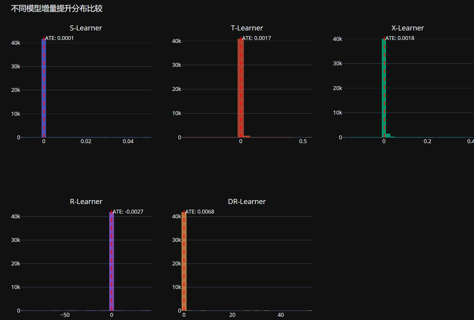
# 计算平均增量提升 (ATE)
ate_results = {}
for name, uplift in uplift_predictions.items():
ate = uplift.mean()
ate_results[name] = ate
print(f"{name} 平均增量提升 (ATE): {ate:.6f}")
# 使用Plotly创建可视化 - 增量提升分布比较
# 创建2行3列的子图布局(因为现在有5个模型)
fig_uplift = make_subplots(rows=2, cols=3, subplot_titles=list(uplift_predictions.keys()))
for i, (name, uplift) in enumerate(uplift_predictions.items()):
row = i // 3 + 1
col = i % 3 + 1
fig_uplift.add_trace(
go.Histogram(
x=uplift,
name=name,
nbinsx=50,
opacity=0.7
),
row=row, col=col
)
fig_uplift.add_vline(
x=ate_results[name],
line_dash="dash",
line_color="red",
annotation_text=f"ATE: {ate_results[name]:.4f}",
annotation_position="top right",
row=row, col=col
)
fig_uplift.update_layout(
title='不同模型增量提升分布比较',
height=800,
showlegend=False
)
fig_uplift.show()
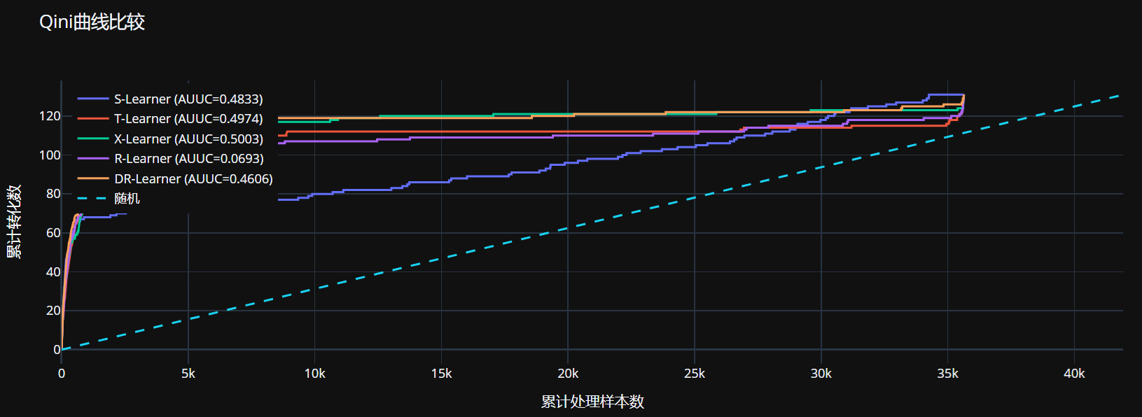
# 评估模型性能 - Qini曲线和AUUC
auuc_results = {}
qini_curves = {}

for name, uplift in uplift_predictions.items():
    # 确保所有数组长度一致
    min_length = min(len(W_test), len(Y_test), len(uplift))

    # 创建包含必要列的DataFrame
    auuc_df = pd.DataFrame({
        'treatment': W_test.values[:min_length],
        'conversion': Y_test.values[:min_length],
        'uplift': uplift[:min_length]
    })

    # 添加模型名称列
    auuc_df['model'] = name

    # 计算AUUC
    auuc_series = auuc_score(auuc_df, outcome_col='conversion', treatment_col='treatment', treatment_effect_col='uplift')

    # 提取AUUC值 - 通常是第一个值
    auuc_value = auuc_series.iloc[0] if isinstance(auuc_series, pd.Series) else auuc_series
    auuc_results[name] = auuc_value
    print(f"{name} AUUC: {auuc_value:.4f}")

    # 计算Qini曲线数据
    qini_df = pd.DataFrame({
        'uplift': uplift[:min_length],
        'treatment': W_test.values[:min_length],
        'conversion': Y_test.values[:min_length]
    })
    qini_df = qini_df.sort_values('uplift', ascending=False)
    qini_df['cumulative_treatment'] = qini_df['treatment'].cumsum()
    qini_df['cumulative_conversion'] = qini_df['conversion'].cumsum()
    qini_curves[name] = qini_df

# 使用Plotly创建Qini曲线比较
fig_qini = go.Figure()

for name, qini_df in qini_curves.items():
    fig_qini.add_trace(go.Scatter(
        x=qini_df['cumulative_treatment'],
        y=qini_df['cumulative_conversion'],
        mode='lines',
        name=f"{name} (AUUC={auuc_results[name]:.4f})"
    ))

# 添加随机线
fig_qini.add_trace(go.Scatter(
    x=[0, len(qini_df)],
    y=[0, qini_df['conversion'].sum()],
    mode='lines',
    name='随机',
    line=dict(dash='dash')
))

fig_qini.update_layout(
    title='Qini曲线比较',
    xaxis_title='累计处理样本数',
    yaxis_title='累计转化数',
    legend=dict(yanchor="top", y=0.99, xanchor="left", x=0.01)
)
fig_qini.show()
S-Learner AUUC: 0.4833
T-Learner AUUC: 0.4974
X-Learner AUUC: 0.5003
R-Learner AUUC: 0.0693
DR-Learner AUUC: 0.4606
# 选择最佳模型(基于AUUC)
best_model_name = max(auuc_results, key=auuc_results.get)
best_uplift = uplift_predictions[best_model_name]
print(f"最佳模型: {best_model_name} (AUUC={auuc_results[best_model_name]:.4f})")

# 创建结果DataFrame用于后续分析
min_length = min(len(W_test), len(Y_test), len(best_uplift))
uplift_df = pd.DataFrame({
    'uplift': best_uplift[:min_length],
    'actual_treatment': W_test.values[:min_length],
    'actual_conversion': Y_test.values[:min_length]
}, index=X_test.index[:min_length])

# 添加原始特征
for col in feature_columns:
    uplift_df[col] = X_test[col].values[:min_length]

# 按增量提升排序
uplift_df_sorted = uplift_df.sort_values('uplift', ascending=False)

# 分析前10%高响应人群
top_10_percent = int(len(uplift_df_sorted) * 0.1)
high_response = uplift_df_sorted.head(top_10_percent)
low_response = uplift_df_sorted.tail(top_10_percent)

print(f"高响应人群 (前10%) 平均增量提升: {high_response['uplift'].mean():.6f}")
print(f"低响应人群 (后10%) 平均增量提升: {low_response['uplift'].mean():.6f}")
最佳模型: X-Learner (AUUC=0.5003)
高响应人群 (前10%) 平均增量提升: 0.013861
低响应人群 (后10%) 平均增量提升: -0.000464
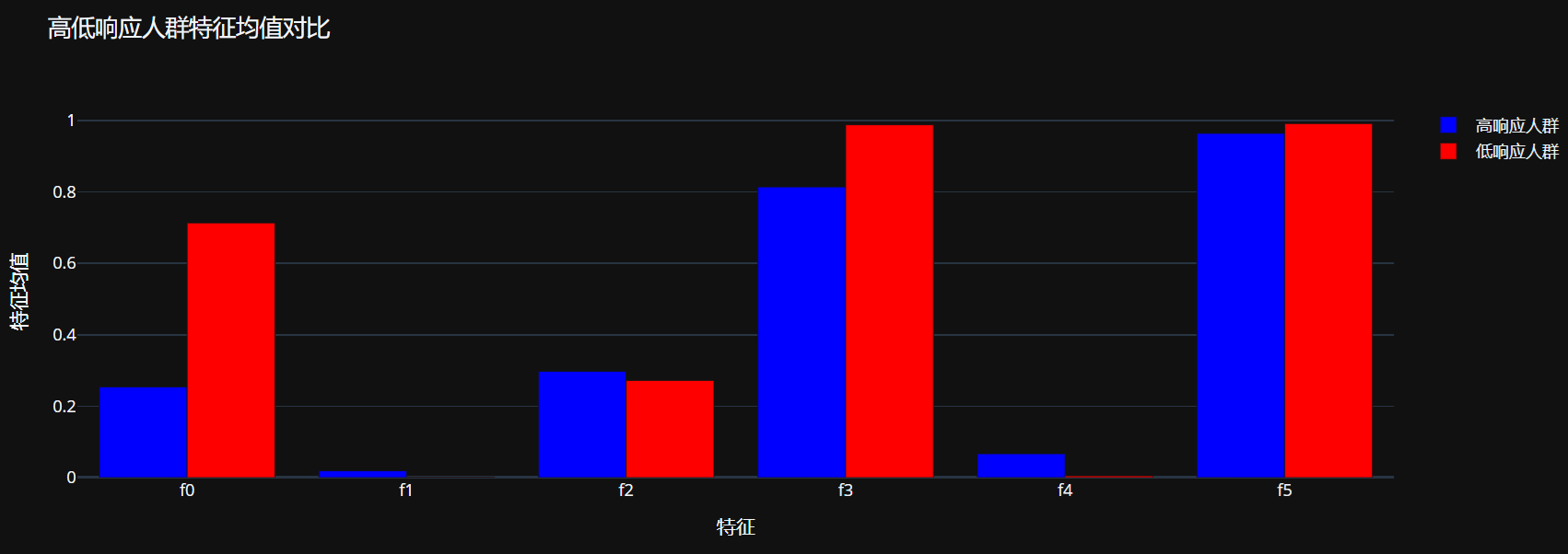
# 使用Plotly创建高低响应人群特征对比可视化
feature_comparison_data = []
for feature in feature_columns[:6]:  # 只展示前6个特征
    feature_comparison_data.append({
        'feature': feature,
        'high_response_mean': high_response[feature].mean(),
        'low_response_mean': low_response[feature].mean()
    })

feature_comparison_df = pd.DataFrame(feature_comparison_data)

# 创建特征对比条形图
fig_features = go.Figure()
fig_features.add_trace(go.Bar(
    x=feature_comparison_df['feature'],
    y=feature_comparison_df['high_response_mean'],
    name='高响应人群',
    marker_color='blue'
))
fig_features.add_trace(go.Bar(
    x=feature_comparison_df['feature'],
    y=feature_comparison_df['low_response_mean'],
    name='低响应人群',
    marker_color='red'
))

fig_features.update_layout(
    title='高低响应人群特征均值对比',
    xaxis_title='特征',
    yaxis_title='特征均值',
    barmode='group'
)

fig_features.show()
# 评估增量提升模型的业务价值
# 模拟只对高响应人群投放广告的场景
targeted_group = high_response.copy()
targeted_group['targeted'] = 1 # 标记为投放目标
# 对照组:随机选择相同数量的人群
control_group = uplift_df_sorted.sample(n=top_10_percent, random_state=42)
control_group['targeted'] = 0 # 标记为非投放目标
# 合并两组数据
simulation_df = pd.concat([targeted_group, control_group])
# 计算业务指标
targeted_conversion_rate = simulation_df[simulation_df['targeted'] == 1]['actual_conversion'].mean()
control_conversion_rate = simulation_df[simulation_df['targeted'] == 0]['actual_conversion'].mean()
print(f"目标组转化率: {targeted_conversion_rate:.6f}")
print(f"对照组转化率: {control_conversion_rate:.6f}")
print(f"提升效果: {(targeted_conversion_rate - control_conversion_rate):.6f}")
print(f"相对提升: {(targeted_conversion_rate - control_conversion_rate)/control_conversion_rate*100:.2f}%")
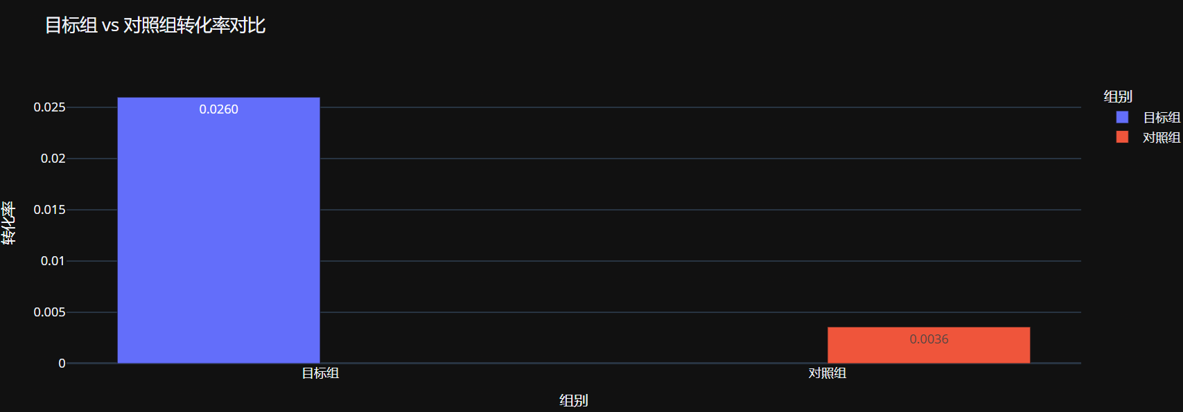
# 使用Plotly创建业务模拟结果可视化
simulation_results = pd.DataFrame({
'group': ['目标组', '对照组'],
'conversion_rate': [targeted_conversion_rate, control_conversion_rate]
})
fig_simulation = px.bar(
simulation_results,
x='group',
y='conversion_rate',
title='目标组 vs 对照组转化率对比',
labels={'conversion_rate': '转化率', 'group': '组别'},
color='group',
text_auto='.4f'
)
fig_simulation.show()
目标组转化率: 0.025996
对照组转化率: 0.003577
提升效果: 0.022418
相对提升: 626.67%
# 特征重要性分析 - 使用最佳模型
if best_model_name == 'S-Learner':
    # S-Learner的特征重要性
    if hasattr(s_learner.learner, 'feature_importances_'):
        feature_importances = s_learner.learner.feature_importances_
        feature_importance = pd.DataFrame({
            'feature': feature_columns + ['treatment'],
            'importance': feature_importances
        }).sort_values('importance', ascending=False)
    else:
        print("警告: S-Learner模型没有特征重要性属性")
        feature_importance = pd.DataFrame({
            'feature': feature_columns + ['treatment'],
            'importance': np.zeros(len(feature_columns) + 1)
        })
elif best_model_name == 'T-Learner':
    # T-Learner的特征重要性 - 取平均
    if hasattr(t_learner.models[1], 'feature_importances_') and hasattr(t_learner.models[0], 'feature_importances_'):
        importance_treatment = t_learner.models[1].feature_importances_
        importance_control = t_learner.models[0].feature_importances_
        avg_importance = (importance_treatment + importance_control) / 2
        feature_importance = pd.DataFrame({
            'feature': feature_columns,
            'importance': avg_importance
        }).sort_values('importance', ascending=False)
    else:
        print("警告: T-Learner模型没有特征重要性属性")
        feature_importance = pd.DataFrame({
            'feature': feature_columns,
            'importance': np.zeros(len(feature_columns))
        })
elif best_model_name == 'X-Learner':
    # X-Learner的特征重要性 - 使用第一个学习器
    feature_importances = None

    # 尝试不同的属性获取特征重要性
    if hasattr(x_learner, 'models_tau_t') and len(x_learner.models_tau_t) > 0:
        # 获取第一个处理组别的模型
        first_group = list(x_learner.models_tau_t.keys())[0]
        model = x_learner.models_tau_t[first_group]
        if hasattr(model, 'feature_importances_'):
            feature_importances = model.feature_importances_
    elif hasattr(x_learner, 'models_mu_t') and len(x_learner.models_mu_t) > 0:
        # 获取第一个处理组别的模型
        first_group = list(x_learner.models_mu_t.keys())[0]
        model = x_learner.models_mu_t[first_group]
        if hasattr(model, 'feature_importances_'):
            feature_importances = model.feature_importances_
    elif hasattr(x_learner, 'learner') and hasattr(x_learner.learner, 'feature_importances_'):
        feature_importances = x_learner.learner.feature_importances_

    if feature_importances is not None:
        feature_importance = pd.DataFrame({
            'feature': feature_columns,
            'importance': feature_importances
        }).sort_values('importance', ascending=False)
    else:
        print("警告: X-Learner模型没有可用的特征重要性属性")
        feature_importance = pd.DataFrame({
            'feature': feature_columns,
            'importance': np.zeros(len(feature_columns))
        })
elif best_model_name == 'R-Learner':
    # R-Learner的特征重要性
    feature_importances = None

    # 尝试多种方法获取特征重要性
    if hasattr(r_learner, 'model') and hasattr(r_learner.model, 'feature_importances_'):
        # 方法1: 直接访问模型
        feature_importances = r_learner.model.feature_importances_
    elif hasattr(r_learner, 'effect_learner') and hasattr(r_learner.effect_learner, 'feature_importances_'):
        # 方法2: 访问effect_learner属性
        feature_importances = r_learner.effect_learner.feature_importances_
    elif hasattr(r_learner, 'outcome_learner') and hasattr(r_learner.outcome_learner, 'feature_importances_'):
        # 方法3: 访问outcome_learner属性
        feature_importances = r_learner.outcome_learner.feature_importances_
    else:
        # 方法4: 使用SHAP值
        try:
            explainer = shap.TreeExplainer(r_learner.model)
            shap_values = explainer.shap_values(X_test)
            feature_importances = np.abs(shap_values).mean(axis=0)
        except:
            # 方法5: 使用排列重要性
            try:
                perm_importance = permutation_importance(
                    r_learner.model, X_test, Y_test,
                    n_repeats=10,
                    random_state=42
                )
                feature_importances = perm_importance.importances_mean
            except:
                print("警告: R-Learner模型没有可用的特征重要性属性")

    if feature_importances is not None:
        feature_importance = pd.DataFrame({
            'feature': feature_columns,
            'importance': feature_importances
        }).sort_values('importance', ascending=False)
    else:
        print("警告: R-Learner模型没有特征重要性属性")
        feature_importance = pd.DataFrame({
            'feature': feature_columns,
            'importance': np.zeros(len(feature_columns))
        })
elif best_model_name == 'DR-Learner':
    # DR-Learner的特征重要性 - 使用结果模型
    if hasattr(dr_learner, 'outcome_learner') and hasattr(dr_learner.outcome_learner, 'feature_importances_'):
        feature_importances = dr_learner.outcome_learner.feature_importances_
        feature_importance = pd.DataFrame({
            'feature': feature_columns,
            'importance': feature_importances
        }).sort_values('importance', ascending=False)
    else:
        print("警告: DR-Learner模型没有特征重要性属性")
        feature_importance = pd.DataFrame({
            'feature': feature_columns,
            'importance': np.zeros(len(feature_columns))
        })

print("特征重要性排序:")
print(feature_importance)
# 使用Plotly创建特征重要性可视化
fig_importance = px.bar(
    feature_importance,
    x='importance',
    y='feature',
    title=f'{best_model_name} 特征重要性',
    orientation='h',
    labels={'importance': '重要性', 'feature': '特征'}
)

fig_importance.show()

# 创建散点图矩阵,展示前4个重要特征与增量提升的关系
top_features = feature_importance.head(4)['feature'].tolist()

if top_features:
    scatter_matrix_data = uplift_df.copy()
    scatter_matrix_data['uplift_group'] = pd.qcut(uplift_df['uplift'], 4, labels=['最低', '低', '高', '最高'])

    fig_scatter = px.scatter_matrix(
        scatter_matrix_data,
        dimensions=top_features,
        color='uplift_group',
        title='前几个重要特征与增量提升的关系',
        opacity=0.5
    )

    fig_scatter.show()
特征重要性排序:
   feature  importance
4       f4    0.190516
10     f10    0.128957
11     f11    0.128275
6       f6    0.124515
2       f2    0.104948
9       f9    0.085479
3       f3    0.066818
8       f8    0.062539
0       f0    0.050294
7       f7    0.026442
5       f5    0.022442
1       f1    0.008775
Tree-based algorithms
# 代码片段1:环境设置和导入
import os
os.environ['CAUSALML_DISABLE_DUECREDIT'] = '1'  # 禁用duecredit

import pandas as pd
import numpy as np
from sklearn.model_selection import train_test_split
from causalml.inference.tree import UpliftTreeClassifier, UpliftRandomForestClassifier
from causalml.metrics import auuc_score, get_cumgain
import plotly.express as px
from sklearn.metrics import auc
import plotly.graph_objects as go
from plotly.subplots import make_subplots

# 设置随机种子确保结果可复现
np.random.seed(42)

print("环境设置完成,库导入成功")

# 代码片段2:数据加载和预处理
def load_and_preprocess_data(file_path='data/criteo-data.csv'):
    """加载并预处理数据"""
    # 加载Criteo数据集
    data = pd.read_csv(file_path)

    # 准备特征和处理变量
    feature_columns = ['f0', 'f1', 'f2', 'f3', 'f4', 'f5', 'f6', 'f7', 'f8', 'f9', 'f10', 'f11']
    X = data[feature_columns]
    W = data['treatment']  # 处理变量:是否分配到实验组
    Y = data['conversion']  # 结果变量:是否转化

    # 数据验证和修复
    print("验证数据质量...")

    # 检查处理变量是否只有0和1
    if not set(W.unique()).issubset({0, 1}):
        print(f"处理变量包含异常值: {set(W.unique())}")
        W = W.map({0: 0, 1: 1}).fillna(0).astype(int)
        print("已修正处理变量")

    # 检查结果变量是否只有0和1
    if not set(Y.unique()).issubset({0, 1}):
        print(f"结果变量包含异常值: {set(Y.unique())}")
        Y = Y.map({0: 0, 1: 1}).fillna(0).astype(int)
        print("已修正结果变量")

    # 检查特征值范围并标准化
    for col in feature_columns:
        min_val = X[col].min()
        max_val = X[col].max()
        if min_val < 0 or max_val > 1:
            print(f"特征 {col} 值范围超出[0,1]: [{min_val}, {max_val}]")
            X[col] = (X[col] - min_val) / (max_val - min_val)
            print(f"已将特征 {col} 标准化到[0,1]范围")

    return X, W, Y, feature_columns

# 执行数据加载和预处理
X, W, Y, feature_columns = load_and_preprocess_data()

print(f"数据加载完成,特征数量: {len(feature_columns)}")
print(f"总样本数: {len(X)}")
print(f"治疗组比例: {W.mean():.4f}")
print(f"总体转化率: {Y.mean():.4f}")

# 代码片段3:数据划分
def split_data(X, W, Y, test_size=0.3, random_state=42):
    """划分训练集和测试集"""
    X_train, X_test, W_train, W_test, Y_train, Y_test = train_test_split(
        X, W, Y, test_size=test_size, random_state=random_state, stratify=Y
    )

    print(f"训练集大小: {X_train.shape[0]}")
    print(f"测试集大小: {X_test.shape[0]}")
    print(f"训练集中转化率: {Y_train.mean():.4f}")
    print(f"测试集中转化率: {Y_test.mean():.4f}")
    print(f"训练集治疗组比例: {W_train.mean():.4f}")
    print(f"测试集治疗组比例: {W_test.mean():.4f}")

    return X_train, X_test, W_train, W_test, Y_train, Y_test

# 执行数据划分
X_train, X_test, W_train, W_test, Y_train, Y_test = split_data(X, W, Y)

# 代码片段4:模型配置和训练
def create_model_configs():
    """创建模型配置字典"""
    base_params = {
        'n_estimators': 100,
        'max_features': 10,
        'random_state': 42,
        'max_depth': 5,
        'min_samples_leaf': 100,
        'min_samples_treatment': 10,
        'n_reg': 100,
        'control_name': '0'
    }

    model_configs = {
        'KL_RF': {'evaluationFunction': 'KL', 'model_class': UpliftRandomForestClassifier},
        'Euclidean_RF': {'evaluationFunction': 'ED', 'model_class': UpliftRandomForestClassifier},
        'Chi_RF': {'evaluationFunction': 'Chi', 'model_class': UpliftRandomForestClassifier},
        'CTS_RF': {'evaluationFunction': 'CTS', 'model_class': UpliftRandomForestClassifier},
        'DDP_RF': {'evaluationFunction': 'DDP', 'model_class': UpliftRandomForestClassifier},
        'IDDP_RF': {'evaluationFunction': 'IDDP', 'model_class': UpliftRandomForestClassifier},
        'Interaction_Tree': {'evaluationFunction': 'IT', 'model_class': UpliftTreeClassifier},
        'Causal_Tree': {'evaluationFunction': 'CIT', 'model_class': UpliftTreeClassifier}
    }

    # 合并基础参数
    for config in model_configs.values():
        config.update(base_params)

    return model_configs

def train_models(model_configs, X_train, W_train, Y_train):
    """训练所有模型"""
    models = {}
    W_train_str = W_train.astype(str)  # 统一转换为字符串

    for name, config in model_configs.items():
        print(f"训练 {name}...")
        try:
            # 创建模型实例
            model_class = config.pop('model_class')
            model = model_class(**config)

            # 训练模型
            model.fit(X_train.values, W_train_str.values, Y_train.values)
            models[name] = model
            print(f"  {name} 训练完成")

        except Exception as e:
            print(f"  {name} 训练失败: {e}")
            models[name] = None

    return models

# 创建模型配置并训练
model_configs = create_model_configs()
models = train_models(model_configs, X_train, W_train, Y_train)

# 过滤掉训练失败的模型
valid_models = {name: model for name, model in models.items() if model is not None}
print(f"\n成功训练模型数量: {len(valid_models)}/{len(model_configs)}")

# 代码片段5:模型预测
def get_uplift_predictions(models, X_test):
    """安全地获取各模型的uplift预测"""
    uplift_predictions = {}

    for name, model in models.items():
        try:
            # 获取预测
            uplift = model.predict(X_test.values)
            print(f"{name} 原始预测形状: {uplift.shape}")

            # 根据情况处理预测结果
            if len(uplift.shape) == 1:
                # 一维数组,直接使用
                uplift_predictions[name] = uplift
            elif uplift.shape[1] == 1:
                # 单列二维数组,展平
                uplift_predictions[name] = uplift.flatten()
            elif uplift.shape[1] == 2:
                # 两列,假设是控制组和治疗组的概率
                uplift_predictions[name] = uplift[:, 1] - uplift[:, 0]
            else:
                # 多列,使用第一列作为uplift(常见情况)
                uplift_predictions[name] = uplift[:, 0]
                print(f"  警告: {name} 输出{uplift.shape[1]}列,使用第一列作为uplift")

            print(f"  {name} uplift范围: [{uplift_predictions[name].min():.4f}, {uplift_predictions[name].max():.4f}]")

        except Exception as e:
            print(f"处理 {name} 时出错: {e}")
            uplift_predictions[name] = np.zeros(len(X_test))  # 返回零数组作为占位符

    return uplift_predictions

# 执行预测
uplift_predictions = get_uplift_predictions(valid_models, X_test)

# 验证预测结果
print("\n预测结果验证:")
for name, uplift in uplift_predictions.items():
print(f"{name}: 形状{uplift.shape}, 空值{np.isnan(uplift).sum()}")

# 代码片段6:评估指标计算
def calculate_robust_auuc(treatment, outcome, uplift, model_name, n_bins=100):
    """针对低转化率数据的稳健AUUC计算方法"""
    try:
        treatment = treatment.copy()
        outcome = outcome.copy()
        uplift = uplift.copy()

        treatment = treatment.astype(int)
        outcome = outcome.astype(int)

        # 按uplift降序排列
        sorted_idx = np.argsort(uplift)[::-1]
        sorted_treatment = treatment.iloc[sorted_idx] if hasattr(treatment, 'iloc') else treatment[sorted_idx]
        sorted_outcome = outcome.iloc[sorted_idx] if hasattr(outcome, 'iloc') else outcome[sorted_idx]

        n = len(treatment)
        bin_size = max(1, n // n_bins)
        cumulative_gain = []

        for i in range(1, n_bins + 1):
            end_idx = min(i * bin_size, n)
            bin_treatment = sorted_treatment[:end_idx]
            bin_outcome = sorted_outcome[:end_idx]

            treatment_mask = (bin_treatment == 1)
            control_mask = (bin_treatment == 0)

            if treatment_mask.sum() > 0 and control_mask.sum() > 0:
                treatment_rate = bin_outcome[treatment_mask].mean()
                control_rate = bin_outcome[control_mask].mean()
                gain = treatment_rate - control_rate
            else:
                gain = 0

            cumulative_gain.append(gain)

        # 计算AUUC(梯形法则)
        x_axis = np.linspace(0, 1, len(cumulative_gain))
        auuc_value = auc(x_axis, cumulative_gain)
        return auuc_value

    except Exception as e:
        print(f"{model_name} 稳健AUUC计算错误: {e}")
        return np.nan

def calculate_simple_qini(treatment, outcome, uplift, model_name):
    """简化的Qini系数计算"""
    try:
        sorted_idx = np.argsort(uplift)[::-1]
        sorted_treatment = treatment.iloc[sorted_idx] if hasattr(treatment, 'iloc') else treatment[sorted_idx]
        sorted_outcome = outcome.iloc[sorted_idx] if hasattr(outcome, 'iloc') else outcome[sorted_idx]

        n = len(treatment)
        qini_curve = []

        for i in range(1, min(101, n)):
            percentile = i / 100.0
            idx = int(n * percentile)

            subset_treatment = sorted_treatment[:idx]
            subset_outcome = sorted_outcome[:idx]

            if (subset_treatment == 1).sum() > 0 and (subset_treatment == 0).sum() > 0:
                treatment_rate = subset_outcome[subset_treatment == 1].mean()
                control_rate = subset_outcome[subset_treatment == 0].mean()
                uplift_value = treatment_rate - control_rate
                qini_curve.append(uplift_value * idx)
            else:
                qini_curve.append(0)

        if len(qini_curve) > 1:
            x_axis = np.linspace(0, 1, len(qini_curve))
            qini_value = auc(x_axis, qini_curve)
        else:
            qini_value = 0

        return qini_value

    except Exception as e:
        print(f"{model_name} Qini计算错误: {e}")
        return np.nan

def calculate_bin_effects(uplift, treatment, outcome, n_bins=10):
    """计算分桶平均效应"""
    try:
        uplift_bins = pd.qcut(uplift, n_bins, duplicates='drop')
        bin_effects = []

        for bin_label in uplift_bins.unique():
            bin_mask = (uplift_bins == bin_label)
            if bin_mask.sum() > 0:
                treatment_rate = outcome[bin_mask & (treatment == 1)].mean() if (bin_mask & (treatment == 1)).sum() > 0 else 0
                control_rate = outcome[bin_mask & (treatment == 0)].mean() if (bin_mask & (treatment == 0)).sum() > 0 else 0
                true_effect = treatment_rate - control_rate
                bin_effects.append(true_effect)

        return np.mean(bin_effects) if len(bin_effects) > 1 else np.nan
    except:
        return np.nan

def evaluate_models(uplift_predictions, W_test, Y_test):
    """评估所有模型性能"""
    metrics_results = {}

    print("计算模型评估指标...")
    for name, uplift in uplift_predictions.items():
        print(f"\n计算 {name} 的指标:")

        # 稳健AUUC
        auuc_robust = calculate_robust_auuc(W_test, Y_test, uplift, name)
        print(f"  稳健AUUC: {auuc_robust:.6f}")

        # Qini系数
        qini = calculate_simple_qini(W_test, Y_test, uplift, name)
        print(f"  Qini系数: {qini:.6f}")

        # 平均uplift
        mean_uplift = np.mean(uplift)
        print(f"  平均uplift: {mean_uplift:.6f}")

        # 分桶平均效应
        bin_effect = calculate_bin_effects(uplift, W_test, Y_test)
        print(f"  分桶平均效应: {bin_effect:.6f}")

        metrics_results[name] = {
            'robust_auuc': auuc_robust,
            'qini': qini,
            'mean_uplift': mean_uplift,
            'bin_effect': bin_effect
        }

    return metrics_results

# 执行模型评估
metrics_results = evaluate_models(uplift_predictions, W_test, Y_test)

# 代码片段7:结果可视化
def create_evaluation_dashboard(metrics_results):
    """创建评估结果仪表板"""
    fig = make_subplots(
        rows=2, cols=2,
        subplot_titles=('稳健AUUC比较', 'Qini系数比较', '平均Uplift比较', '分桶平均效应比较'),
        specs=[[{"type": "bar"}, {"type": "bar"}],
               [{"type": "bar"}, {"type": "bar"}]]
    )

    models = list(metrics_results.keys())

    # 稳健AUUC
    auuc_values = [metrics['robust_auuc'] for metrics in metrics_results.values()]
    sorted_idx = np.argsort(auuc_values)[::-1]
    fig.add_trace(
        go.Bar(x=[models[i] for i in sorted_idx], y=[auuc_values[i] for i in sorted_idx],
               name='稳健AUUC', marker_color='blue'),
        row=1, col=1
    )

    # Qini系数
    qini_values = [metrics['qini'] for metrics in metrics_results.values()]
    sorted_idx_qini = np.argsort(qini_values)[::-1]
    fig.add_trace(
        go.Bar(x=[models[i] for i in sorted_idx_qini], y=[qini_values[i] for i in sorted_idx_qini],
               name='Qini系数', marker_color='orange'),
        row=1, col=2
    )

    # 平均uplift
    uplift_values = [metrics['mean_uplift'] for metrics in metrics_results.values()]
    sorted_idx_uplift = np.argsort(uplift_values)[::-1]
    fig.add_trace(
        go.Bar(x=[models[i] for i in sorted_idx_uplift], y=[uplift_values[i] for i in sorted_idx_uplift],
               name='平均Uplift', marker_color='green'),
        row=2, col=1
    )

    # 分桶效应
    effect_values = [metrics['bin_effect'] for metrics in metrics_results.values() if not np.isnan(metrics['bin_effect'])]
    effect_models = [model for i, model in enumerate(models) if not np.isnan(list(metrics_results.values())[i]['bin_effect'])]

    if effect_values:
        sorted_idx_effect = np.argsort(effect_values)[::-1]
        fig.add_trace(
            go.Bar(x=[effect_models[i] for i in sorted_idx_effect], y=[effect_values[i] for i in sorted_idx_effect],
                   name='分桶平均效应', marker_color='red'),
            row=2, col=2
        )

    fig.update_layout(height=800, title_text="模型综合评估仪表板", showlegend=False)
    fig.update_xaxes(tickangle=45)

    return fig

def create_ranking_table(metrics_results):
    """创建模型排名表"""
    ranking_data = []
    for model_name, metrics in metrics_results.items():
        ranking_data.append({
            'Model': model_name,
            'Robust_AUUC': metrics['robust_auuc'],
            'Qini': metrics['qini'],
            'Mean_Uplift': metrics['mean_uplift'],
            'Bin_Effect': metrics['bin_effect'] if not np.isnan(metrics['bin_effect']) else 'N/A'
        })

    ranking_df = pd.DataFrame(ranking_data)
    ranking_df = ranking_df.sort_values('Robust_AUUC', ascending=False)

    # 计算综合评分
    try:
        for col in ['Robust_AUUC', 'Qini', 'Mean_Uplift']:
            if ranking_df[col].apply(lambda x: isinstance(x, (int, float))).all():
                max_val = ranking_df[col].max()
                min_val = ranking_df[col].min()
                if max_val > min_val:
                    ranking_df[f'{col}_Normalized'] = (ranking_df[col] - min_val) / (max_val - min_val)
                else:
                    ranking_df[f'{col}_Normalized'] = 0.5

        weights = {'Robust_AUUC_Normalized': 0.4, 'Qini_Normalized': 0.4, 'Mean_Uplift_Normalized': 0.2}
        ranking_df['Composite_Score'] = 0

        for metric, weight in weights.items():
            if metric in ranking_df.columns:
                ranking_df['Composite_Score'] += ranking_df[metric] * weight

        ranking_df = ranking_df.sort_values('Composite_Score', ascending=False)

    except Exception as e:
        print(f"综合评分计算失败: {e}")

    return ranking_df

# 创建可视化
dashboard_fig = create_evaluation_dashboard(metrics_results)
dashboard_fig.show()

# 显示排名表
ranking_df = create_ranking_table(metrics_results)
print("模型综合排名:")
display(ranking_df)
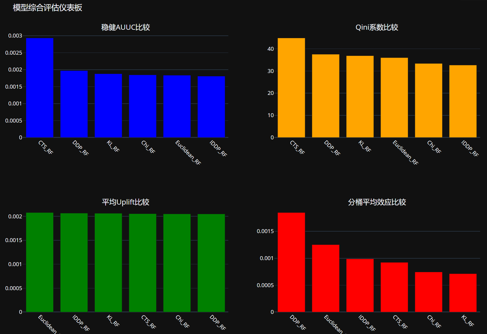
# 代码片段8:特征重要性分析和业务价值评估
def analyze_feature_importance(models, feature_columns, model_name='KL_RF'):
    """分析特征重要性"""
    if model_name in models and hasattr(models[model_name], 'feature_importances_'):
        feature_importances = models[model_name].feature_importances_
        feature_importance_df = pd.DataFrame({
            'feature': feature_columns,
            'importance': feature_importances
        }).sort_values('importance', ascending=False)

        print(f"{model_name}特征重要性排序:")
        print(feature_importance_df)

        fig_importance = px.bar(
            feature_importance_df,
            x='importance',
            y='feature',
            orientation='h',
            title=f'{model_name}特征重要性',
            labels={'importance': '重要性', 'feature': '特征'},
            color='importance',
            color_continuous_scale='Viridis'
        )
        fig_importance.update_layout(yaxis={'categoryorder': 'total ascending'})
        fig_importance.show()

        return feature_importance_df
    else:
        print(f"{model_name}模型不支持特征重要性分析")
        return None

def analyze_business_value(uplift_predictions, W_test, Y_test, X_test, feature_columns, top_percent=0.1):
    """分析业务价值"""
    # 选择最佳模型
    valid_results = {k: v for k, v in metrics_results.items() if not np.isnan(v['robust_auuc'])}
    if not valid_results:
        print("没有有效的模型结果")
        return

    best_model_name = max(valid_results, key=lambda x: valid_results[x]['robust_auuc'])
    best_uplift = uplift_predictions[best_model_name]

    print(f"最佳模型: {best_model_name} (AUUC={valid_results[best_model_name]['robust_auuc']:.4f})")

    # 创建结果DataFrame
    uplift_df = pd.DataFrame({
        'uplift': best_uplift,
        'actual_treatment': W_test.values,
        'actual_conversion': Y_test.values
    }, index=X_test.index)

    # 添加原始特征
    for col in feature_columns:
        uplift_df[col] = X_test[col].values

    # 按增量提升排序
    uplift_df_sorted = uplift_df.sort_values('uplift', ascending=False)

    # 分析高低响应人群
    top_n = int(len(uplift_df_sorted) * top_percent)
    high_response = uplift_df_sorted.head(top_n)
    low_response = uplift_df_sorted.tail(top_n)

    print(f"\n高响应人群 (前{top_percent*100}%) 平均增量提升: {high_response['uplift'].mean():.6f}")
    print(f"低响应人群 (后{top_percent*100}%) 平均增量提升: {low_response['uplift'].mean():.6f}")

    # 业务价值评估
    targeted_conversion = high_response[high_response['actual_treatment'] == 1]['actual_conversion'].mean()
    control_conversion = low_response[low_response['actual_treatment'] == 1]['actual_conversion'].mean()

    print(f"\n业务价值分析:")
    print(f"目标组转化率: {targeted_conversion:.6f}")
    print(f"对照组转化率: {control_conversion:.6f}")
    print(f"提升效果: {(targeted_conversion - control_conversion):.6f}")
    if control_conversion > 0:
        print(f"相对提升: {(targeted_conversion - control_conversion)/control_conversion*100:.2f}%")

    # 创建特征分布对比图
    if len(feature_columns) >= 6:
        fig_dist = make_subplots(rows=2, cols=3, subplot_titles=feature_columns[:6])

        for i, feature in enumerate(feature_columns[:6]):
            row = i // 3 + 1
            col = i % 3 + 1

            fig_dist.add_trace(
                go.Histogram(x=high_response[feature], name='高响应人群', marker_color='blue', opacity=0.7),
                row=row, col=col
            )

            fig_dist.add_trace(
                go.Histogram(x=low_response[feature], name='低响应人群', marker_color='red', opacity=0.7),
                row=row, col=col
            )

        fig_dist.update_layout(title='高低响应人群特征分布对比', height=600, showlegend=False)
        fig_dist.show()

    return uplift_df_sorted, high_response, low_response

# 执行特征重要性分析
feature_importance_df = analyze_feature_importance(valid_models, feature_columns)

# 执行业务价值分析
uplift_df_sorted, high_response, low_response = analyze_business_value(
    uplift_predictions, W_test, Y_test, X_test, feature_columns
)
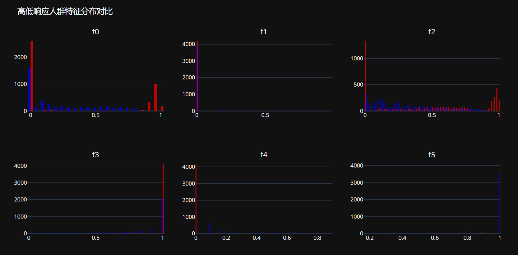
# 代码片段9:最终总结和结果保存
def generate_summary_report(metrics_results, uplift_predictions, models):
    """生成总结报告"""
    print("=" * 60)
    print("模型训练和评估总结报告")
    print("=" * 60)

    print(f"\n1. 模型训练情况:")
    print(f"   成功训练模型: {len(models)}个")
    print(f"   有效预测模型: {len(uplift_predictions)}个")

    print(f"\n2. 数据概况:")
    print(f"   总样本数: {len(X)}")
    print(f"   训练集样本: {len(X_train)}")
    print(f"   测试集样本: {len(X_test)}")
    print(f"   总体转化率: {Y.mean():.4f}")
    print(f"   治疗组比例: {W.mean():.4f}")

    print(f"\n3. 最佳模型排名 (按稳健AUUC):")
    valid_models = {k: v for k, v in metrics_results.items() if not np.isnan(v['robust_auuc'])}
    sorted_models = sorted(valid_models.items(), key=lambda x: x[1]['robust_auuc'], reverse=True)

    for i, (model_name, metrics) in enumerate(sorted_models[:3], 1):
        print(f"   第{i}名: {model_name} (AUUC: {metrics['robust_auuc']:.4f})")

    print(f"\n4. 关键发现:")
    if sorted_models:
        best_model = sorted_models[0]
        print(f"   • 最佳模型: {best_model[0]}")
        print(f"   • 最佳AUUC: {best_model[1]['robust_auuc']:.4f}")
        print(f"   • 平均Uplift: {best_model[1]['mean_uplift']:.4f}")

    print(f"\n5. 建议:")
    print("   • 建议使用最佳模型进行后续的营销策略制定")
    print("   • 可根据特征重要性调整营销资源分配")
    print("   • 建议对高响应人群进行重点营销")

# 生成总结报告
generate_summary_report(metrics_results, uplift_predictions, valid_models)

# 可选:保存重要结果
try:
    # 保存模型评估结果
    results_df = pd.DataFrame.from_dict(metrics_results, orient='index')
    results_df.to_csv('model_evaluation_results.csv', encoding='utf-8-sig')
    print(f"\n评估结果已保存至: model_evaluation_results.csv")

    # 保存最佳模型的预测结果
    best_model_name = max(metrics_results, key=lambda x: metrics_results[x]['robust_auuc'])
    best_predictions = pd.DataFrame({
        'uplift': uplift_predictions[best_model_name],
        'actual_treatment': W_test.values,
        'actual_conversion': Y_test.values
    })
    best_predictions.to_csv('best_model_predictions.csv', encoding='utf-8-sig')
    print(f"最佳模型预测结果已保存至: best_model_predictions.csv")

except Exception as e:
    print(f"保存结果时出错: {e}")

print("\n所有分析完成!")
Neural network based algorithms
# 代码片段4.1:神经网络算法导入和配置(修复版)
import torch
import torch.nn as nn
import torch.optim as optim
from torch.utils.data import DataLoader, TensorDataset
import warnings
warnings.filterwarnings('ignore')

print("神经网络算法库导入完成")

def check_gpu_availability():
    """检查GPU可用性"""
    if torch.cuda.is_available():
        device = torch.device('cuda')
        print(f"GPU可用: {torch.cuda.get_device_name(0)}")
    else:
        device = torch.device('cpu')
        print("使用CPU进行训练")
    return device

device = check_gpu_availability()

# 代码片段4.2:数据预处理适配神经网络
def prepare_nn_data(X_train, X_test, W_train, W_test, Y_train, Y_test):
    """为神经网络算法准备数据"""
    # 转换为PyTorch张量
    X_train_tensor = torch.FloatTensor(X_train.values)
    X_test_tensor = torch.FloatTensor(X_test.values)
    W_train_tensor = torch.FloatTensor(W_train.values).unsqueeze(1)
    W_test_tensor = torch.FloatTensor(W_test.values).unsqueeze(1)
    Y_train_tensor = torch.FloatTensor(Y_train.values).unsqueeze(1)
    Y_test_tensor = torch.FloatTensor(Y_test.values).unsqueeze(1)

    # 创建数据加载器
    train_dataset = TensorDataset(X_train_tensor, W_train_tensor, Y_train_tensor)
    train_loader = DataLoader(train_dataset, batch_size=512, shuffle=True)

    print(f"训练数据形状: {X_train_tensor.shape}")
    print(f"测试数据形状: {X_test_tensor.shape}")
    print(f"批次大小: 512")

    return train_loader, X_train_tensor, X_test_tensor, W_train_tensor, W_test_tensor, Y_train_tensor, Y_test_tensor

# 准备神经网络数据
train_loader, X_train_tensor, X_test_tensor, W_train_tensor, W_test_tensor, Y_train_tensor, Y_test_tensor = prepare_nn_data(
    X_train, X_test, W_train, W_test, Y_train, Y_test
)

# 代码片段4.3:CEVAE模型独立实现
class CEVAE(nn.Module):
    """CEVAE (Causal Effect Variational Autoencoder) 独立实现"""
    def __init__(self, input_dim, latent_dim=20, hidden_dim=200):
        super(CEVAE, self).__init__()
        self.input_dim = input_dim
        self.latent_dim = latent_dim
        self.hidden_dim = hidden_dim

        # 编码器网络 (x, t) -> z
        self.encoder = nn.Sequential(
            nn.Linear(input_dim + 1, hidden_dim),  # +1 for treatment
            nn.ReLU(),
            nn.Linear(hidden_dim, hidden_dim),
            nn.ReLU(),
        )

        # 潜在变量分布参数
        self.z_mu = nn.Linear(hidden_dim, latent_dim)
        self.z_logvar = nn.Linear(hidden_dim, latent_dim)

        # 解码器网络 (z, t) -> (x, y)
        self.decoder = nn.Sequential(
            nn.Linear(latent_dim + 1, hidden_dim),  # +1 for treatment
            nn.ReLU(),
            nn.Linear(hidden_dim, hidden_dim),
            nn.ReLU(),
            nn.Linear(hidden_dim, input_dim + 1),  # +1 for outcome
        )

    def encode(self, x, t):
        """编码输入到潜在空间"""
        inputs = torch.cat([x, t], dim=1)
        hidden = self.encoder(inputs)
        z_mu = self.z_mu(hidden)
        z_logvar = self.z_logvar(hidden)
        return z_mu, z_logvar

    def reparameterize(self, mu, logvar):
        """重参数化技巧"""
        std = torch.exp(0.5 * logvar)
        eps = torch.randn_like(std)
        return mu + eps * std

    def decode(self, z, t):
        """从潜在空间解码"""
        inputs = torch.cat([z, t], dim=1)
        reconstruction = self.decoder(inputs)
        x_recon = reconstruction[:, :-1]  # 重建特征
        y_recon = torch.sigmoid(reconstruction[:, -1:])  # 预测结果概率
        return x_recon, y_recon

    def forward(self, x, t, y):
        """前向传播"""
        # 编码到潜在空间
        z_mu, z_logvar = self.encode(x, t)
        z = self.reparameterize(z_mu, z_logvar)

        # 从潜在空间解码
        x_recon, y_recon = self.decode(z, t)

        return x_recon, y_recon, z_mu, z_logvar

def cevae_loss_function(x, x_recon, y, y_recon, mu, logvar, beta=1.0):
    """CEVAE损失函数 - 重建损失 + KL散度"""
    # 特征重建损失 (MSE)
    reconstruction_loss_x = nn.MSELoss()(x_recon, x)

    # 结果重建损失 (BCE)
    reconstruction_loss_y = nn.BCELoss()(y_recon, y)

    # 总重建损失
    reconstruction_loss = reconstruction_loss_x + reconstruction_loss_y

    # KL散度损失
    kl_divergence = -0.5 * torch.sum(1 + logvar - mu.pow(2) - logvar.exp()) / x.size(0)

    # 总损失
    total_loss = reconstruction_loss + beta * kl_divergence

    return total_loss, reconstruction_loss, kl_divergence

def train_cevae_model(model, train_loader, epochs=100, learning_rate=1e-3):
    """训练CEVAE模型"""
    optimizer = optim.Adam(model.parameters(), lr=learning_rate)
    model.train()

    train_losses = []
    reconstruction_losses = []
    kl_losses = []

    print("开始训练CEVAE模型...")
    for epoch in range(epochs):
        epoch_total_loss = 0
        epoch_recon_loss = 0
        epoch_kl_loss = 0

        for batch_x, batch_t, batch_y in train_loader:
            # 移动到设备
            batch_x = batch_x.to(device)
            batch_t = batch_t.to(device)
            batch_y = batch_y.to(device)

            # 清零梯度
            optimizer.zero_grad()

            # 前向传播
            x_recon, y_recon, mu, logvar = model(batch_x, batch_t, batch_y)

            # 计算损失
            total_loss, recon_loss, kl_loss = cevae_loss_function(
                batch_x, x_recon, batch_y, y_recon, mu, logvar
            )

            # 反向传播
            total_loss.backward()
            optimizer.step()

            # 累计损失
            epoch_total_loss += total_loss.item()
            epoch_recon_loss += recon_loss.item()
            epoch_kl_loss += kl_loss.item()

        # 计算平均损失
        avg_total_loss = epoch_total_loss / len(train_loader)
        avg_recon_loss = epoch_recon_loss / len(train_loader)
        avg_kl_loss = epoch_kl_loss / len(train_loader)

        train_losses.append(avg_total_loss)
        reconstruction_losses.append(avg_recon_loss)
        kl_losses.append(avg_kl_loss)

        # 每20轮打印一次进度
        if epoch % 20 == 0 or epoch == epochs - 1:
            print(f"Epoch {epoch:3d}/{epochs} | Total Loss: {avg_total_loss:.4f} | "
                  f"Recon Loss: {avg_recon_loss:.4f} | KL Loss: {avg_kl_loss:.4f}")

    print("CEVAE模型训练完成!")
    return train_losses, reconstruction_losses, kl_losses

def predict_cevae_uplift(model, X_test, device=device):
    """使用训练好的CEVAE模型预测uplift"""
    model.eval()

    with torch.no_grad():
        # 确保输入数据在正确设备上
        X_test_tensor = X_test.to(device) if isinstance(X_test, torch.Tensor) else torch.FloatTensor(X_test).to(device)

        # 创建治疗组和对照组的治疗变量
        batch_size = X_test_tensor.size(0)
        t0 = torch.zeros(batch_size, 1).to(device)  # 对照组
        t1 = torch.ones(batch_size, 1).to(device)   # 治疗组

        # 预测潜在结果
        _, y0_pred, _, _ = model(X_test_tensor, t0, torch.zeros(batch_size, 1).to(device))
        _, y1_pred, _, _ = model(X_test_tensor, t1, torch.zeros(batch_size, 1).to(device))

        # 计算uplift (ITE)
        uplift = y1_pred - y0_pred

        return uplift.cpu().numpy().flatten()

# 创建并训练CEVAE模型
print("初始化CEVAE模型...")
cevae_model = CEVAE(
    input_dim=X_train.shape[1],
    latent_dim=20,
    hidden_dim=100
).to(device)

# 训练模型
cevae_losses, recon_losses, kl_losses = train_cevae_model(
    cevae_model,
    train_loader,
    epochs=100,
    learning_rate=1e-3
)

# 预测uplift
cevae_uplift = predict_cevae_uplift(cevae_model, X_test_tensor)
print(f"CEVAE uplift预测范围: [{cevae_uplift.min():.4f}, {cevae_uplift.max():.4f}]")

# 代码片段4.4:DragonNet模型独立实现
class DragonNet(nn.Module):
    """DragonNet模型独立实现"""
    def __init__(self, input_dim, hidden_dim=200, output_dim=1):
        super(DragonNet, self).__init__()
        self.input_dim = input_dim
        self.hidden_dim = hidden_dim

        # 共享的特征提取层
        self.shared_network = nn.Sequential(
            nn.Linear(input_dim, hidden_dim),
            nn.ReLU(),
            nn.Dropout(0.1),
            nn.Linear(hidden_dim, hidden_dim),
            nn.ReLU(),
            nn.Dropout(0.1),
            nn.Linear(hidden_dim, hidden_dim),
            nn.ReLU(),
        )

        # 治疗倾向评分头
        self.propensity_head = nn.Sequential(
            nn.Linear(hidden_dim, hidden_dim // 2),
            nn.ReLU(),
            nn.Linear(hidden_dim // 2, 1),
            nn.Sigmoid()  # 输出概率值
        )

        # 结果预测头
        self.outcome_head = nn.Sequential(
            nn.Linear(hidden_dim + 1, hidden_dim),  # +1 for treatment
            nn.ReLU(),
            nn.Linear(hidden_dim, hidden_dim // 2),
            nn.ReLU(),
            nn.Linear(hidden_dim // 2, output_dim),
            nn.Sigmoid()  # 输出概率值
        )

    def forward(self, x, t):
        """前向传播"""
        # 共享特征提取
        shared_features = self.shared_network(x)

        # 倾向评分预测
        propensity_score = self.propensity_head(shared_features)

        # 结果预测(包含治疗信息)
        outcome_features = torch.cat([shared_features, t], dim=1)
        outcome_pred = self.outcome_head(outcome_features)

        return propensity_score, outcome_pred

def dragonnet_loss_function(propensity_pred, outcome_pred, treatment_true, outcome_true, alpha=0.5):
    """DragonNet多任务损失函数"""
    # 倾向评分损失(二元交叉熵)
    propensity_loss = nn.BCELoss()(propensity_pred, treatment_true)

    # 结果预测损失(二元交叉熵)
    outcome_loss = nn.BCELoss()(outcome_pred, outcome_true)

    # 倾向评分平衡正则化(减少治疗组选择的偏差)
    propensity_mean = propensity_pred.mean()
    balance_regularization = torch.mean((propensity_pred - propensity_mean) ** 2)

    # 总损失(加权组合)
    total_loss = outcome_loss + alpha * propensity_loss + 0.1 * balance_regularization

    return total_loss, outcome_loss, propensity_loss

def train_dragonnet_model(model, train_loader, epochs=100, learning_rate=1e-3):
    """训练DragonNet模型"""
    optimizer = optim.Adam(model.parameters(), lr=learning_rate)
    model.train()

    total_losses = []
    outcome_losses = []
    propensity_losses = []

    print("开始训练DragonNet模型...")
    for epoch in range(epochs):
        epoch_total_loss = 0
        epoch_outcome_loss = 0
        epoch_propensity_loss = 0

        for batch_x, batch_t, batch_y in train_loader:
            # 移动到设备
            batch_x = batch_x.to(device)
            batch_t = batch_t.to(device)
            batch_y = batch_y.to(device)

            # 清零梯度
            optimizer.zero_grad()

            # 前向传播
            propensity_pred, outcome_pred = model(batch_x, batch_t)

            # 计算损失
            total_loss, outcome_loss, propensity_loss = dragonnet_loss_function(
                propensity_pred, outcome_pred, batch_t, batch_y
            )

            # 反向传播
            total_loss.backward()
            optimizer.step()

            # 累计损失
            epoch_total_loss += total_loss.item()
            epoch_outcome_loss += outcome_loss.item()
            epoch_propensity_loss += propensity_loss.item()

        # 计算平均损失
        avg_total_loss = epoch_total_loss / len(train_loader)
        avg_outcome_loss = epoch_outcome_loss / len(train_loader)
        avg_propensity_loss = epoch_propensity_loss / len(train_loader)

        total_losses.append(avg_total_loss)
        outcome_losses.append(avg_outcome_loss)
        propensity_losses.append(avg_propensity_loss)

        # 每20轮打印一次进度
        if epoch % 20 == 0 or epoch == epochs - 1:
            print(f"Epoch {epoch:3d}/{epochs} | Total Loss: {avg_total_loss:.4f} | "
                  f"Outcome Loss: {avg_outcome_loss:.4f} | Propensity Loss: {avg_propensity_loss:.4f}")

    print("DragonNet模型训练完成!")
    return total_losses, outcome_losses, propensity_losses

def predict_dragonnet_uplift(model, X_test, device=device):
    """使用训练好的DragonNet模型预测uplift"""
    model.eval()

    with torch.no_grad():
        # 确保输入数据在正确设备上
        X_test_tensor = X_test.to(device) if isinstance(X_test, torch.Tensor) else torch.FloatTensor(X_test).to(device)

        # 创建治疗组和对照组的治疗变量
        batch_size = X_test_tensor.size(0)
        t0 = torch.zeros(batch_size, 1).to(device)  # 对照组
        t1 = torch.ones(batch_size, 1).to(device)   # 治疗组

        # 预测潜在结果
        _, y0_pred = model(X_test_tensor, t0)
        _, y1_pred = model(X_test_tensor, t1)

        # 计算uplift (ITE)
        uplift = y1_pred - y0_pred

        return uplift.cpu().numpy().flatten()

# 创建并训练DragonNet模型
print("初始化DragonNet模型...")
dragonnet_model = DragonNet(
    input_dim=X_train.shape[1],
    hidden_dim=100
).to(device)

# 训练模型
dragonnet_losses, outcome_losses, propensity_losses = train_dragonnet_model(
    dragonnet_model,
    train_loader,
    epochs=100,
    learning_rate=1e-3
)

# 预测uplift
dragonnet_uplift = predict_dragonnet_uplift(dragonnet_model, X_test_tensor)
print(f"DragonNet uplift预测范围: [{dragonnet_uplift.min():.4f}, {dragonnet_uplift.max():.4f}]")

# 代码片段4.5:集成神经网络模型到现有框架
def create_nn_model_configs():
    """创建神经网络模型配置"""
    nn_models = {
        'CEVAE': cevae_model,
        'DragonNet': dragonnet_model
    }

    nn_uplift_predictions = {
        'CEVAE': cevae_uplift,
        'DragonNet': dragonnet_uplift
    }

    return nn_models, nn_uplift_predictions

# 创建神经网络模型配置
nn_models, nn_uplift_predictions = create_nn_model_configs()

print(f"神经网络模型创建完成:")
print(f"- CEVAE: uplift范围 [{cevae_uplift.min():.4f}, {cevae_uplift.max():.4f}]")
print(f"- DragonNet: uplift范围 [{dragonnet_uplift.min():.4f}, {dragonnet_uplift.max():.4f}]")

# 代码片段4.6:神经网络模型评估(使用之前定义的函数)
def evaluate_nn_models(nn_uplift_predictions, W_test, Y_test):
    """评估神经网络模型性能"""
    nn_metrics_results = {}

    print("评估神经网络模型...")
    for name, uplift in nn_uplift_predictions.items():
        print(f"\n计算 {name} 的指标:")

        # 稳健AUUC
        auuc_robust = calculate_robust_auuc(W_test, Y_test, uplift, name)
        print(f"  稳健AUUC: {auuc_robust:.6f}")

        # Qini系数
        qini = calculate_simple_qini(W_test, Y_test, uplift, name)
        print(f"  Qini系数: {qini:.6f}")

        # 平均uplift
        mean_uplift = np.mean(uplift)
        print(f"  平均uplift: {mean_uplift:.6f}")

        # 分桶平均效应
        bin_effect = calculate_bin_effects(uplift, W_test, Y_test)
        print(f"  分桶平均效应: {bin_effect:.6f}")

        nn_metrics_results[name] = {
            'robust_auuc': auuc_robust,
            'qini': qini,
            'mean_uplift': mean_uplift,
            'bin_effect': bin_effect
        }

    return nn_metrics_results

# 评估神经网络模型
nn_metrics_results = evaluate_nn_models(nn_uplift_predictions, W_test, Y_test)

print(f"\n神经网络模型评估完成!")

# 代码片段4.7:神经网络模型可视化
def create_nn_training_plots(cevae_losses, dragonnet_losses):
    """创建神经网络训练过程可视化"""
    fig = make_subplots(
        rows=1, cols=2,
        subplot_titles=('CEVAE训练损失', 'DragonNet训练损失')
    )

    # CEVAE损失曲线
    fig.add_trace(
        go.Scatter(x=list(range(len(cevae_losses))), y=cevae_losses,
                  name='CEVAE损失', line=dict(color='blue')),
        row=1, col=1
    )

    # DragonNet损失曲线
    fig.add_trace(
        go.Scatter(x=list(range(len(dragonnet_losses))), y=dragonnet_losses,
                  name='DragonNet损失', line=dict(color='red')),
        row=1, col=2
    )

    fig.update_layout(
        title='神经网络模型训练过程',
        xaxis_title='训练轮次',
        yaxis_title='损失值',
        height=400
    )

    return fig

# 创建训练过程可视化
training_plot = create_nn_training_plots(cevae_losses, dragonnet_losses)
training_plot.show()
# 代码片段4.8:更新主评估流程以包含神经网络模型
# 注意:这里需要确保之前的代码片段已经定义了 metrics_results 和 uplift_predictions

# 将神经网络模型添加到现有模型字典中
all_models = {**valid_models, **nn_models}
all_uplift_predictions = {**uplift_predictions, **nn_uplift_predictions}
all_metrics_results = {**metrics_results, **nn_metrics_results}

print(f"所有模型整合完成:")
print(f"传统模型: {len(valid_models)}个")
print(f"神经网络模型: {len(nn_models)}个")
print(f"总计: {len(all_models)}个模型")

# 代码片段4.9:创建包含神经网络模型的综合评估仪表板
def create_comprehensive_dashboard(all_metrics_results):
    """创建包含所有模型的综合评估仪表板"""
    fig = make_subplots(
        rows=2, cols=2,
        subplot_titles=('稳健AUUC比较', 'Qini系数比较', '平均Uplift比较', '分桶平均效应比较'),
        specs=[[{"type": "bar"}, {"type": "bar"}],
               [{"type": "bar"}, {"type": "bar"}]]
    )

    models = list(all_metrics_results.keys())

    # 区分传统模型和神经网络模型的颜色
    colors = []
    for model in models:
        if model in ['CEVAE', 'DragonNet']:
            colors.append('red')  # 神经网络模型用红色
        else:
            colors.append('blue')  # 传统模型用蓝色

    # 稳健AUUC
    auuc_values = [all_metrics_results[model]['robust_auuc'] for model in models]
    sorted_idx = np.argsort(auuc_values)[::-1]

    fig.add_trace(
        go.Bar(x=[models[i] for i in sorted_idx], y=[auuc_values[i] for i in sorted_idx],
               marker_color=[colors[i] for i in sorted_idx],
               name='稳健AUUC'),
        row=1, col=1
    )

    # Qini系数
    qini_values = [all_metrics_results[model]['qini'] for model in models]
    sorted_idx_qini = np.argsort(qini_values)[::-1]

    fig.add_trace(
        go.Bar(x=[models[i] for i in sorted_idx_qini], y=[qini_values[i] for i in sorted_idx_qini],
               marker_color=[colors[i] for i in sorted_idx_qini],
               name='Qini系数'),
        row=1, col=2
    )

    # 平均uplift
    uplift_values = [all_metrics_results[model]['mean_uplift'] for model in models]
    sorted_idx_uplift = np.argsort(uplift_values)[::-1]

    fig.add_trace(
        go.Bar(x=[models[i] for i in sorted_idx_uplift], y=[uplift_values[i] for i in sorted_idx_uplift],
               marker_color=[colors[i] for i in sorted_idx_uplift],
               name='平均Uplift'),
        row=2, col=1
    )

    # 分桶效应
    effect_data = [(model, all_metrics_results[model]['bin_effect'])
                   for model in models if not np.isnan(all_metrics_results[model]['bin_effect'])]

    if effect_data:
        effect_models, effect_values = zip(*effect_data)
        effect_colors = ['red' if model in ['CEVAE', 'DragonNet'] else 'blue' for model in effect_models]

        sorted_idx_effect = np.argsort(effect_values)[::-1]
        fig.add_trace(
            go.Bar(x=[effect_models[i] for i in sorted_idx_effect],
                   y=[effect_values[i] for i in sorted_idx_effect],
                   marker_color=[effect_colors[i] for i in sorted_idx_effect],
                   name='分桶平均效应'),
            row=2, col=2
        )

    fig.update_layout(
        height=800,
        title_text="包含神经网络模型的综合评估仪表板",
        showlegend=False,
        annotations=[
            dict(
                x=0.5, y=-0.15,
                xref="paper", yref="paper",
                text="蓝色: 传统模型 | 红色: 神经网络模型",
                showarrow=False,
                font=dict(size=12)
            )
        ]
    )
    fig.update_xaxes(tickangle=45)

    return fig

# 创建综合仪表板
comprehensive_dashboard = create_comprehensive_dashboard(all_metrics_results)
comprehensive_dashboard.show()
# 代码片段4.10:模型比较和总结
def compare_model_performance(all_metrics_results):
    """比较传统模型和神经网络模型的性能"""
    traditional_models = [name for name in all_metrics_results.keys() if name not in ['CEVAE', 'DragonNet']]
    nn_models = [name for name in all_metrics_results.keys() if name in ['CEVAE', 'DragonNet']]

    print("模型性能比较分析:")
    print("=" * 50)

    if traditional_models:
        traditional_auuc = [all_metrics_results[name]['robust_auuc'] for name in traditional_models]
        avg_traditional = np.mean(traditional_auuc)
        print(f"传统模型平均AUUC: {avg_traditional:.6f}")
        print(f"最佳传统模型: {max(traditional_models, key=lambda x: all_metrics_results[x]['robust_auuc'])}")

    if nn_models:
        nn_auuc = [all_metrics_results[name]['robust_auuc'] for name in nn_models]
        avg_nn = np.mean(nn_auuc)
        print(f"神经网络模型平均AUUC: {avg_nn:.6f}")
        print(f"最佳神经网络模型: {max(nn_models, key=lambda x: all_metrics_results[x]['robust_auuc'])}")

    if traditional_models and nn_models:
        improvement = ((avg_nn - avg_traditional) / avg_traditional) * 100
        print(f"神经网络模型相比传统模型的改进: {improvement:.2f}%")

        if improvement > 0:
            print("结论: 神经网络模型在平均性能上优于传统模型")
        else:
            print("结论: 传统模型在平均性能上优于神经网络模型")

    # 创建性能比较箱线图
    fig = go.Figure()

    if traditional_models:
        fig.add_trace(go.Box(
            y=[all_metrics_results[name]['robust_auuc'] for name in traditional_models],
            name='传统模型',
            boxpoints='all',
            jitter=0.3,
            marker_color='blue'
        ))

    if nn_models:
        fig.add_trace(go.Box(
            y=[all_metrics_results[name]['robust_auuc'] for name in nn_models],
            name='神经网络模型',
            boxpoints='all',
            jitter=0.3,
            marker_color='red'
        ))

    fig.update_layout(
        title='传统模型 vs 神经网络模型性能分布',
        yaxis_title='稳健AUUC',
        showlegend=True
    )

    return fig

# 执行模型比较
comparison_plot = compare_model_performance(all_metrics_results)
comparison_plot.show()

print("\n神经网络算法集成完成!")
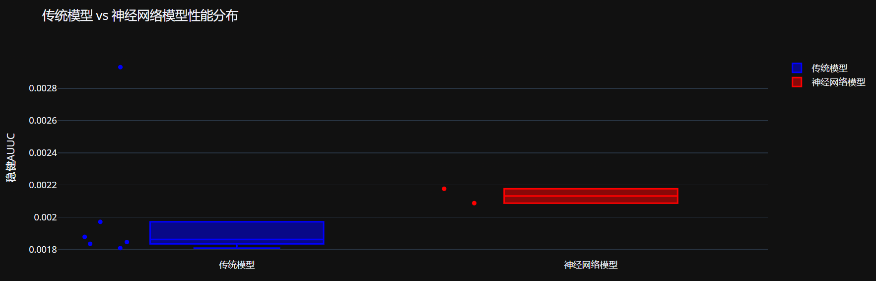
Instrumental variables algorithms
# 代码片段5.1:工具变量算法导入和配置
import numpy as np
import pandas as pd
from sklearn.linear_model import LinearRegression
from sklearn.ensemble import RandomForestRegressor
from sklearn.preprocessing import StandardScaler
from sklearn.model_selection import train_test_split
import warnings
warnings.filterwarnings('ignore')

print("工具变量算法库导入完成")

# 代码片段5.2:工具变量数据准备和模拟
def prepare_iv_data(X, W, Y, instrument_strength=0.5, random_state=42):
    """
    准备工具变量数据
    在实际应用中,工具变量应该是外部变量,这里我们模拟生成
    """
    np.random.seed(random_state)

    # 假设我们有一个有效的工具变量Z
    n_samples = len(X)

    # 从特征中创建一个与处理变量相关的工具变量
    # 在实际应用中,工具变量应该满足:
    # 1. 与处理变量相关
    # 2. 只通过处理变量影响结果变量
    # 3. 与误差项不相关

    # 使用部分特征创建工具变量
    if X.shape[1] >= 3:
        # 选择前3个特征来创建工具变量
        selected_features = X.iloc[:, :3].values
        # 创建与处理变量相关的工具变量
        Z = np.dot(selected_features, np.random.randn(3)) + np.random.normal(0, 0.1, n_samples)

        # 调整工具变量强度
        Z = instrument_strength * Z + (1 - instrument_strength) * np.random.normal(0, 1, n_samples)
    else:
        # 如果特征不足,使用随机工具变量
        Z = np.random.normal(0, 1, n_samples)

    # 将工具变量添加到数据中
    X_with_iv = X.copy()
    X_with_iv['instrument'] = Z

    print(f"工具变量数据准备完成:")
    print(f"工具变量与处理变量的相关性: {np.corrcoef(Z, W)[0,1]:.4f}")
    print(f"工具变量与结果变量的相关性: {np.corrcoef(Z, Y)[0,1]:.4f}")

    return X_with_iv, Z

# 准备工具变量数据
X_with_iv, Z = prepare_iv_data(X, W, Y, instrument_strength=0.7)

# 划分训练集和测试集(包含工具变量)
X_train_iv, X_test_iv, W_train_iv, W_test_iv, Y_train_iv, Y_test_iv, Z_train, Z_test = train_test_split(
    X_with_iv, W, Y, Z, test_size=0.3, random_state=42, stratify=Y
)

print(f"工具变量数据划分完成:")
print(f"训练集大小: {X_train_iv.shape[0]}")
print(f"测试集大小: {X_test_iv.shape[0]}")

# 代码片段5.3:2-Stage Least Squares (2SLS) 实现
class TwoStageLeastSquares:
    """2-Stage Least Squares (2SLS) 实现"""

    def __init__(self, first_stage_model=None, second_stage_model=None):
        """
        初始化2SLS模型

        Parameters:
        first_stage_model: 第一阶段模型(预测处理变量)
        second_stage_model: 第二阶段模型(预测结果变量)
        """
        self.first_stage_model = first_stage_model or LinearRegression()
        self.second_stage_model = second_stage_model or LinearRegression()
        self.is_fitted = False

    def fit(self, X, Z, W, Y):
        """
        拟合2SLS模型

        Parameters:
        X: 特征矩阵(协变量)
        Z: 工具变量
        W: 处理变量
        Y: 结果变量
        """
        # 确保输入为numpy数组
        if hasattr(X, 'values'):
            X = X.values
        if hasattr(Z, 'values'):
            Z = Z.values
        if hasattr(W, 'values'):
            W = W.values
        if hasattr(Y, 'values'):
            Y = Y.values

        Z = Z.reshape(-1, 1) if Z.ndim == 1 else Z
        W = W.reshape(-1, 1) if W.ndim == 1 else W
        Y = Y.reshape(-1, 1) if Y.ndim == 1 else Y

        # 第一阶段:使用工具变量Z和协变量X预测处理变量W
        first_stage_features = np.column_stack([X, Z]) if X.ndim > 1 else np.column_stack([X.reshape(-1, 1), Z])

        self.first_stage_model.fit(first_stage_features, W)
        W_hat = self.first_stage_model.predict(first_stage_features)

        # 第二阶段:使用预测的处理变量W_hat和协变量X预测结果变量Y
        second_stage_features = np.column_stack([X, W_hat]) if X.ndim > 1 else np.column_stack([X.reshape(-1, 1), W_hat])

        self.second_stage_model.fit(second_stage_features, Y)

        self.is_fitted = True
        self.first_stage_coef_ = self.first_stage_model.coef_
        self.second_stage_coef_ = self.second_stage_model.coef_

        print("2SLS模型训练完成")
        print(f"第一阶段系数: {self.first_stage_coef_.flatten()}")
        print(f"第二阶段系数: {self.second_stage_coef_.flatten()}")

        return self

    def predict_ite(self, X, Z):
        """
        预测个体处理效应(ITE)

        Parameters:
        X: 特征矩阵
        Z: 工具变量

        Returns:
        ite: 个体处理效应
        """
        if not self.is_fitted:
            raise ValueError("模型尚未训练,请先调用fit方法")

        if hasattr(X, 'values'):
            X = X.values
        if hasattr(Z, 'values'):
            Z = Z.values

        Z = Z.reshape(-1, 1) if Z.ndim == 1 else Z

        # 预测处理变量
        first_stage_features = np.column_stack([X, Z]) if X.ndim > 1 else np.column_stack([X.reshape(-1, 1), Z])
        W_hat = self.first_stage_model.predict(first_stage_features)

        # 预测潜在结果
        # Y(0): W = 0
        W_0 = np.zeros_like(W_hat)
        second_stage_features_0 = np.column_stack([X, W_0]) if X.ndim > 1 else np.column_stack([X.reshape(-1, 1), W_0])
        Y_0 = self.second_stage_model.predict(second_stage_features_0)

        # Y(1): W = 1
        W_1 = np.ones_like(W_hat)
        second_stage_features_1 = np.column_stack([X, W_1]) if X.ndim > 1 else np.column_stack([X.reshape(-1, 1), W_1])
        Y_1 = self.second_stage_model.predict(second_stage_features_1)

        # 计算ITE
        ite = Y_1 - Y_0

        return ite.flatten()

    def predict_uplift(self, X, Z):
        """预测uplift(ITE的别名)"""
        return self.predict_ite(X, Z)

def evaluate_2sls_model(model, X_test, Z_test, W_test, Y_test):
    """评估2SLS模型性能"""
    # 预测ITE
    ite_pred = model.predict_ite(X_test, Z_test)

    # 基本统计
    print("2SLS模型评估:")
    print(f"ITE预测范围: [{ite_pred.min():.4f}, {ite_pred.max():.4f}]")
    print(f"平均ITE: {ite_pred.mean():.4f}")

    # 计算第一阶段预测的R²
    first_stage_features = np.column_stack([X_test.values, Z_test]) if hasattr(X_test, 'values') else np.column_stack([X_test, Z_test])
    W_pred = model.first_stage_model.predict(first_stage_features)
    first_stage_r2 = 1 - np.sum((W_test - W_pred.flatten()) ** 2) / np.sum((W_test - np.mean(W_test)) ** 2)
    print(f"第一阶段R²: {first_stage_r2:.4f}")

    return ite_pred

# 创建并训练2SLS模型
print("训练2SLS模型...")
tsls_model = TwoStageLeastSquares(
    first_stage_model=LinearRegression(),
    second_stage_model=LinearRegression()
)

# 训练模型(使用训练集)
tsls_model.fit(
    X_train_iv.drop('instrument', axis=1),  # 协变量(不包括工具变量)
    Z_train,                                # 工具变量
    W_train_iv,                            # 处理变量
    Y_train_iv                             # 结果变量
)

# 评估模型
tsls_uplift = evaluate_2sls_model(
    tsls_model,
    X_test_iv.drop('instrument', axis=1),
    Z_test,
    W_test_iv,
    Y_test_iv
)

print("2SLS模型完成")

# 代码片段5.4:Doubly Robust Instrumental Variable (DRIV) Learner 实现(修复版)
class DRIVLearner:
    """Doubly Robust Instrumental Variable (DRIV) Learner 实现"""

    def __init__(self, n_splits=3):
        """
        初始化DRIV学习器

        Parameters:
        n_splits: 交叉验证折数
        """
        self.n_splits = n_splits
        self.is_fitted = False
        self.late_ = None

    def fit(self, X, Z, W, Y):
        """
        拟合DRIV模型

        Parameters:
        X: 特征矩阵(协变量)
        Z: 工具变量
        W: 处理变量
        Y: 结果变量
        """
        from sklearn.model_selection import KFold
        from sklearn.ensemble import RandomForestRegressor
        from sklearn.linear_model import LinearRegression

        # 确保输入为numpy数组并处理形状
        X = X.values if hasattr(X, 'values') else X
        Z = Z.values if hasattr(Z, 'values') else Z
        W = W.values if hasattr(W, 'values') else W
        Y = Y.values if hasattr(Y, 'values') else Y

        # 确保正确的形状
        if Z.ndim == 1:
            Z = Z.reshape(-1, 1)
        if W.ndim == 1:
            W = W.reshape(-1, 1)
        if Y.ndim == 1:
            Y = Y.reshape(-1, 1)

        n_samples = X.shape[0]

        # 创建KFold分割
        kf = KFold(n_splits=self.n_splits, shuffle=True, random_state=42)
        indices = list(kf.split(X))

        print("开始DRIV交叉拟合...")

        # 初始化预测数组
        W_hat_Z = np.zeros(n_samples)
        W_hat_X = np.zeros(n_samples)
        Y_hat_X = np.zeros(n_samples)
        Z_residual = np.zeros(n_samples)

        for train_idx, test_idx in indices:
            # 获取训练和测试数据
            X_train, X_test = X[train_idx], X[test_idx]
            Z_train, Z_test = Z[train_idx], Z[test_idx]
            W_train, W_test = W[train_idx], W[test_idx]
            Y_train, Y_test = Y[train_idx], Y[test_idx]

            # 确保形状正确
            if Z_train.ndim == 1:
                Z_train = Z_train.reshape(-1, 1)
            if Z_test.ndim == 1:
                Z_test = Z_test.reshape(-1, 1)
            if W_train.ndim == 1:
                W_train = W_train.reshape(-1, 1)
            if W_test.ndim == 1:
                W_test = W_test.reshape(-1, 1)
            if Y_train.ndim == 1:
                Y_train = Y_train.reshape(-1, 1)
            if Y_test.ndim == 1:
                Y_test = Y_test.reshape(-1, 1)

            # 第一阶段:预测处理变量W给定工具变量Z和协变量X
            features_treatment = np.column_stack([X_train, Z_train.reshape(-1, 1)]) if X_train.ndim > 1 else np.column_stack([X_train.reshape(-1, 1), Z_train.reshape(-1, 1)])
            treatment_model = RandomForestRegressor(n_estimators=50, random_state=42)
            treatment_model.fit(features_treatment, W_train.flatten())

            # 预测测试集
            features_test = np.column_stack([X_test, Z_test.reshape(-1, 1)]) if X_test.ndim > 1 else np.column_stack([X_test.reshape(-1, 1), Z_test.reshape(-1, 1)])
            W_hat_Z[test_idx] = treatment_model.predict(features_test)

            # 预测处理变量W仅给定协变量X
            treatment_model_X = RandomForestRegressor(n_estimators=50, random_state=42)
            treatment_model_X.fit(X_train, W_train.flatten())
            W_hat_X[test_idx] = treatment_model_X.predict(X_test)

            # 预测结果变量Y仅给定协变量X
            outcome_model = RandomForestRegressor(n_estimators=50, random_state=42)
            outcome_model.fit(X_train, Y_train.flatten())
            Y_hat_X[test_idx] = outcome_model.predict(X_test)

            # 计算工具变量残差
            iv_model = LinearRegression()
            iv_model.fit(X_train, Z_train.flatten())
            Z_pred = iv_model.predict(X_test)
            Z_residual[test_idx] = Z_test.flatten() - Z_pred

        # 计算残差
        W_residual = W.flatten() - W_hat_X
        Y_residual = Y.flatten() - Y_hat_X

        # 构建最终特征:工具变量残差和处理变量残差的交互
        final_features = (Z_residual * W_residual).reshape(-1, 1)

        # 最终阶段:估计局部平均处理效应(LATE)
        final_model = LinearRegression()
        final_model.fit(final_features, Y_residual)

        self.is_fitted = True
        self.late_ = final_model.coef_[0]

        print("DRIV模型训练完成")
        print(f"估计的局部平均处理效应(LATE): {self.late_:.4f}")

        return self

    def predict_ite(self, X, Z):
        """
        预测个体处理效应

        Parameters:
        X: 特征矩阵
        Z: 工具变量

        Returns:
        ite: 个体处理效应(对于DRIV,通常返回常数LATE)
        """
        if not self.is_fitted:
            raise ValueError("模型尚未训练,请先调用fit方法")

        # 确保输入为numpy数组
        X = X.values if hasattr(X, 'values') else X
        Z = Z.values if hasattr(Z, 'values') else Z

        n_samples = X.shape[0] if X.ndim > 1 else len(X)

        # DRIV通常估计的是局部平均处理效应(LATE),对于所有个体返回相同的值
        ite = np.full(n_samples, self.late_)

        return ite

    def predict_uplift(self, X, Z):
        """预测uplift"""
        return self.predict_ite(X, Z)

def evaluate_driv_model(model, X_test, Z_test, W_test, Y_test):
    """评估DRIV模型性能"""
    # 预测ITE
    ite_pred = model.predict_ite(X_test, Z_test)

    print("DRIV模型评估:")
    print(f"估计的LATE: {model.late_:.4f}")
    print(f"ITE预测范围: [{ite_pred.min():.4f}, {ite_pred.max():.4f}]")

    # 计算工具变量相关性
    Z_test_flat = Z_test.flatten() if hasattr(Z_test, 'flatten') else Z_test
    W_test_flat = W_test.flatten() if hasattr(W_test, 'flatten') else W_test
    iv_strength = np.corrcoef(Z_test_flat, W_test_flat)[0, 1]
    print(f"工具变量强度(与处理变量的相关性): {iv_strength:.4f}")

    return ite_pred

# 创建并训练DRIV模型
print("训练DRIV模型...")
driv_model = DRIVLearner(n_splits=3)

# 准备数据
X_train_data = X_train_iv.drop('instrument', axis=1).values if hasattr(X_train_iv, 'drop') else X_train_iv
Z_train_data = Z_train.values if hasattr(Z_train, 'values') else Z_train
W_train_data = W_train_iv.values if hasattr(W_train_iv, 'values') else W_train_iv
Y_train_data = Y_train_iv.values if hasattr(Y_train_iv, 'values') else Y_train_iv

# 训练模型
driv_model.fit(X_train_data, Z_train_data, W_train_data, Y_train_data)

# 准备测试数据
X_test_data = X_test_iv.drop('instrument', axis=1).values if hasattr(X_test_iv, 'drop') else X_test_iv
Z_test_data = Z_test.values if hasattr(Z_test, 'values') else Z_test
W_test_data = W_test_iv.values if hasattr(W_test_iv, 'values') else W_test_iv
Y_test_data = Y_test_iv.values if hasattr(Y_test_iv, 'values') else Y_test_iv

# 评估模型
driv_uplift = evaluate_driv_model(
    driv_model,
    X_test_data,
    Z_test_data,
    W_test_data,
    Y_test_data
)

print("DRIV模型完成")

# 代码片段5.5:工具变量模型集成
def create_iv_model_configs():
    """创建工具变量模型配置"""
    iv_models = {
        '2SLS': tsls_model,
        'DRIV': driv_model
    }

    iv_uplift_predictions = {
        '2SLS': tsls_uplift,
        'DRIV': driv_uplift
    }

    return iv_models, iv_uplift_predictions

# 创建工具变量模型配置
iv_models, iv_uplift_predictions = create_iv_model_configs()

print(f"工具变量模型创建完成:")
print(f"- 2SLS: uplift范围 [{tsls_uplift.min():.4f}, {tsls_uplift.max():.4f}]")
print(f"- DRIV: uplift范围 [{driv_uplift.min():.4f}, {driv_uplift.max():.4f}]")

# 代码片段5.6:工具变量模型评估
def evaluate_iv_models(iv_uplift_predictions, W_test, Y_test, Z_test):
    """评估工具变量模型性能"""
    iv_metrics_results = {}

    print("评估工具变量模型...")
    for name, uplift in iv_uplift_predictions.items():
        print(f"\n计算 {name} 的指标:")

        # 稳健AUUC
        auuc_robust = calculate_robust_auuc(W_test, Y_test, uplift, name)
        print(f"  稳健AUUC: {auuc_robust:.6f}")

        # Qini系数
        qini = calculate_simple_qini(W_test, Y_test, uplift, name)
        print(f"  Qini系数: {qini:.6f}")

        # 平均uplift
        mean_uplift = np.mean(uplift)
        print(f"  平均uplift: {mean_uplift:.6f}")

        # 分桶平均效应
        bin_effect = calculate_bin_effects(uplift, W_test, Y_test)
        print(f"  分桶平均效应: {bin_effect:.6f}")

        # 工具变量特定指标
        iv_strength = np.corrcoef(Z_test, W_test)[0, 1] if Z_test is not None else 0
        print(f"  工具变量强度: {iv_strength:.6f}")

        iv_metrics_results[name] = {
            'robust_auuc': auuc_robust,
            'qini': qini,
            'mean_uplift': mean_uplift,
            'bin_effect': bin_effect,
            'iv_strength': iv_strength
        }

    return iv_metrics_results

# 评估工具变量模型
iv_metrics_results = evaluate_iv_models(iv_uplift_predictions, W_test_iv, Y_test_iv, Z_test)

print(f"\n工具变量模型评估完成!")
Treatment optimization algorithms
# 代码片段6.1:治疗优化算法导入和配置
import numpy as np
import pandas as pd
from sklearn.linear_model import LogisticRegression
from sklearn.ensemble import RandomForestClassifier, RandomForestRegressor
from sklearn.metrics import precision_recall_curve, roc_curve, auc
import plotly.express as px
import plotly.graph_objects as go
from plotly.subplots import make_subplots

print("治疗优化算法库导入完成")

# 代码片段6.2:Counterfactual Unit Selection (CUS) 实现
class CounterfactualUnitSelector:
    """
    反事实单元选择器
    用于识别哪些个体最有可能从治疗中受益
    """

    def __init__(self, uplift_model, threshold_strategy='top_k', cost_benefit_ratio=1.0):
        """
        初始化反事实单元选择器

        Parameters:
        uplift_model: 已训练的uplift模型
        threshold_strategy: 阈值策略 ('top_k', 'quantile', 'absolute')
        cost_benefit_ratio: 成本效益比,用于计算最优阈值
        """
        self.uplift_model = uplift_model
        self.threshold_strategy = threshold_strategy
        self.cost_benefit_ratio = cost_benefit_ratio
        self.threshold_ = None
        self.selected_units_ = None

    def fit(self, X, uplift_scores, treatment_cost=1.0, conversion_value=10.0):
        """
        拟合选择器,确定最优阈值

        Parameters:
        X: 特征矩阵
        uplift_scores: uplift预测分数
        treatment_cost: 治疗成本
        conversion_value: 转化价值
        """
        self.treatment_cost = treatment_cost
        self.conversion_value = conversion_value

        # 计算最优阈值
        if self.threshold_strategy == 'top_k':
            # 基于预算约束选择前k%的个体
            self.threshold_ = np.percentile(uplift_scores, 80)  # 默认选择前20%
        elif self.threshold_strategy == 'quantile':
            # 基于分位数选择
            self.threshold_ = np.percentile(uplift_scores, 75)  # 选择前25%
        elif self.threshold_strategy == 'absolute':
            # 基于绝对uplift值选择
            self.threshold_ = 0.0  # 默认选择uplift>0的个体
        elif self.threshold_strategy == 'optimal':
            # 基于成本效益比计算最优阈值
            self.threshold_ = self._calculate_optimal_threshold(uplift_scores)
        else:
            raise ValueError(f"未知的阈值策略: {self.threshold_strategy}")

        print(f"选择阈值: {self.threshold_:.4f} (策略: {self.threshold_strategy})")
        return self

    def _calculate_optimal_threshold(self, uplift_scores):
        """基于成本效益比计算最优阈值"""
        # 计算不同阈值下的预期收益
        thresholds = np.linspace(uplift_scores.min(), uplift_scores.max(), 100)
        expected_values = []

        for threshold in thresholds:
            selected_mask = uplift_scores >= threshold
            n_selected = selected_mask.sum()

            if n_selected == 0:
                expected_values.append(0)
                continue

            # 预期收益 = 选择的个体数 * (平均uplift * 转化价值 - 治疗成本)
            avg_uplift_selected = uplift_scores[selected_mask].mean()
            expected_value = n_selected * (avg_uplift_selected * self.conversion_value - self.treatment_cost)
            expected_values.append(expected_value)

        # 找到最大化预期收益的阈值
        optimal_idx = np.argmax(expected_values)
        optimal_threshold = thresholds[optimal_idx]

        print(f"最优阈值: {optimal_threshold:.4f}, 最大预期收益: {expected_values[optimal_idx]:.2f}")
        return optimal_threshold

    def select_units(self, X, uplift_scores=None):
        """
        选择应该接受治疗的单元

        Parameters:
        X: 特征矩阵
        uplift_scores: uplift预测分数(如果为None,则使用模型预测)

        Returns:
        selected_indices: 被选中的单元索引
        selection_scores: 选择分数
        """
        if uplift_scores is None:
            # 使用模型预测uplift
            uplift_scores = self.uplift_model.predict(X.values) if hasattr(X, 'values') else self.uplift_model.predict(X)

            # 处理不同模型的输出格式
            if uplift_scores.ndim > 1 and uplift_scores.shape[1] >= 2:
                uplift_scores = uplift_scores[:, 1] - uplift_scores[:, 0]
            elif uplift_scores.ndim > 1:
                uplift_scores = uplift_scores.flatten()

        # 应用阈值选择单元
        selected_mask = uplift_scores >= self.threshold_
        selected_indices = np.where(selected_mask)[0]

        self.selected_units_ = {
            'indices': selected_indices,
            'scores': uplift_scores[selected_mask],
            'count': len(selected_indices),
            'selection_rate': len(selected_indices) / len(uplift_scores)
        }

        print(f"选择了 {len(selected_indices)}/{len(uplift_scores)} 个单元 ({self.selected_units_['selection_rate']*100:.1f}%)")
        print(f"选中单元的平均uplift: {uplift_scores[selected_mask].mean():.4f}")

        return selected_indices, uplift_scores

    def evaluate_selection(self, X, W, Y, selected_indices=None):
        """
        评估选择策略的性能

        Parameters:
        X: 特征矩阵
        W: 真实治疗分配
        Y: 真实结果
        selected_indices: 选中的单元索引(如果为None,使用最近的选择)

        Returns:
        evaluation_metrics: 评估指标字典
        """
        if selected_indices is None:
            if self.selected_units_ is None:
                raise ValueError("尚未选择单元,请先调用select_units方法")
            selected_indices = self.selected_units_['indices']

        # 创建选择指示器
        n_samples = len(X) if hasattr(X, '__len__') else X.shape[0]
        selection = np.zeros(n_samples, dtype=bool)
        selection[selected_indices] = True

        # 计算指标
        metrics = {}

        # 1. 选择率
        metrics['selection_rate'] = selection.mean()

        # 2. 选中群体的平均uplift(如果可用)
        if hasattr(self, 'uplift_model'):
            uplift_scores = self.uplift_model.predict(X.values) if hasattr(X, 'values') else self.uplift_model.predict(X)
            if uplift_scores.ndim > 1 and uplift_scores.shape[1] >= 2:
                uplift_scores = uplift_scores[:, 1] - uplift_scores[:, 0]
            metrics['avg_uplift_selected'] = uplift_scores[selection].mean()
            metrics['avg_uplift_not_selected'] = uplift_scores[~selection].mean()

        # 3. 实际治疗组和对照组的转化率
        treatment_mask = (W == 1) if hasattr(W, 'values') else (W == 1)
        control_mask = (W == 0) if hasattr(W, 'values') else (W == 0)

        # 选中群体中的转化率
        selected_treatment = selection & treatment_mask
        selected_control = selection & control_mask

        if selected_treatment.sum() > 0:
            metrics['conversion_rate_selected_treatment'] = Y[selected_treatment].mean()
        else:
            metrics['conversion_rate_selected_treatment'] = 0

        if selected_control.sum() > 0:
            metrics['conversion_rate_selected_control'] = Y[selected_control].mean()
        else:
            metrics['conversion_rate_selected_control'] = 0

        # 4. 预期收益
        n_selected = selection.sum()
        expected_uplift = metrics.get('avg_uplift_selected', 0)
        metrics['expected_value'] = n_selected * (expected_uplift * self.conversion_value - self.treatment_cost)

        # 5. 如果可能,计算真实uplift
        if treatment_mask.sum() > 0 and control_mask.sum() > 0:
            # 选中群体的真实uplift
            selected_treatment_rate = Y[selection & treatment_mask].mean() if (selection & treatment_mask).sum() > 0 else 0
            selected_control_rate = Y[selection & control_mask].mean() if (selection & control_mask).sum() > 0 else 0
            metrics['true_uplift_selected'] = selected_treatment_rate - selected_control_rate

            # 未选中群体的真实uplift
            not_selected_treatment_rate = Y[~selection & treatment_mask].mean() if (~selection & treatment_mask).sum() > 0 else 0
            not_selected_control_rate = Y[~selection & control_mask].mean() if (~selection & control_mask).sum() > 0 else 0
            metrics['true_uplift_not_selected'] = not_selected_treatment_rate - not_selected_control_rate

        print("选择策略评估结果:")
        for key, value in metrics.items():
            print(f"  {key}: {value:.4f}")

        return metrics

# 使用最佳模型创建反事实单元选择器
def create_counterfactual_unit_selector(best_model, X_train, W_train, Y_train, strategy='optimal'):
    """创建反事实单元选择器"""
    print("创建反事实单元选择器...")

    # 使用训练数据拟合选择器
    uplift_scores_train = best_model.predict(X_train.values) if hasattr(X_train, 'values') else best_model.predict(X_train)

    # 处理不同模型的输出格式
    if uplift_scores_train.ndim > 1 and uplift_scores_train.shape[1] >= 2:
        uplift_scores_train = uplift_scores_train[:, 1] - uplift_scores_train[:, 0]
    elif uplift_scores_train.ndim > 1:
        uplift_scores_train = uplift_scores_train.flatten()

    # 创建选择器
    selector = CounterfactualUnitSelector(
        uplift_model=best_model,
        threshold_strategy=strategy,
        cost_benefit_ratio=1.0
    )

    # 拟合选择器(确定最优阈值)
    selector.fit(
        X_train,
        uplift_scores_train,
        treatment_cost=1.0,  # 假设治疗成本为1
        conversion_value=10.0  # 假设转化价值为10
    )

    return selector

# 创建选择器(使用之前确定的最佳模型)
best_model_name = max(metrics_results, key=lambda x: metrics_results[x]['robust_auuc'])
best_model = valid_models[best_model_name]

print(f"使用最佳模型进行单元选择: {best_model_name}")
cus_selector = create_counterfactual_unit_selector(best_model, X_train, W_train, Y_train, strategy='optimal')

# 代码片段6.3:Counterfactual Value Estimator (CVE) 实现
class CounterfactualValueEstimator:
    """
    反事实价值估计器
    用于估计不同治疗策略的预期价值
    """

    def __init__(self, uplift_model, outcome_model=None):
        """
        初始化反事实价值估计器

        Parameters:
        uplift_model: 已训练的uplift模型
        outcome_model: 结果预测模型(可选)
        """
        self.uplift_model = uplift_model
        self.outcome_model = outcome_model
        self.value_estimates_ = None

    def estimate_value(self, X, treatment_strategy, treatment_cost=1.0, conversion_value=10.0,
                     baseline_strategy=None, n_samples=1000):
        """
        估计治疗策略的预期价值

        Parameters:
        X: 特征矩阵
        treatment_strategy: 治疗策略函数,输入特征返回治疗概率
        treatment_cost: 治疗成本
        conversion_value: 转化价值
        baseline_strategy: 基线策略(用于计算增量价值)
        n_samples: 蒙特卡洛模拟的样本数

        Returns:
        value_estimates: 价值估计字典
        """
        # 预测uplift
        uplift_scores = self.uplift_model.predict(X.values) if hasattr(X, 'values') else self.uplift_model.predict(X)

        # 处理不同模型的输出格式
        if uplift_scores.ndim > 1 and uplift_scores.shape[1] >= 2:
            uplift_scores = uplift_scores[:, 1] - uplift_scores[:, 0]
        elif uplift_scores.ndim > 1:
            uplift_scores = uplift_scores.flatten()

        n_units = len(uplift_scores)

        # 应用治疗策略
        if callable(treatment_strategy):
            # 策略函数
            treatment_probs = treatment_strategy(X)
        elif isinstance(treatment_strategy, (int, float)):
            # 固定概率
            treatment_probs = np.full(n_units, treatment_strategy)
        elif treatment_strategy == 'optimal':
            # 基于uplift的最优策略
            treatment_probs = (uplift_scores > 0).astype(float)
        else:
            raise ValueError(f"不支持的治疗策略类型: {type(treatment_strategy)}")

        # 蒙特卡洛模拟
        monte_carlo_results = self._monte_carlo_simulation(
            uplift_scores, treatment_probs, treatment_cost, conversion_value, n_samples
        )

        # 计算价值指标
        value_estimates = {
            'expected_value': monte_carlo_results['expected_value'],
            'expected_cost': monte_carlo_results['expected_cost'],
            'expected_conversions': monte_carlo_results['expected_conversions'],
            'expected_profit': monte_carlo_results['expected_value'] - monte_carlo_results['expected_cost'],
            'treatment_rate': treatment_probs.mean(),
            'avg_uplift_treated': np.mean(uplift_scores * treatment_probs) / treatment_probs.mean() if treatment_probs.mean() > 0 else 0,
            'value_per_unit': (monte_carlo_results['expected_value'] - monte_carlo_results['expected_cost']) / n_units
        }

        # 如果有基线策略,计算增量价值
        if baseline_strategy is not None:
            baseline_value = self.estimate_value(
                X, baseline_strategy, treatment_cost, conversion_value, None, n_samples
            )['expected_value']
            value_estimates['incremental_value'] = value_estimates['expected_value'] - baseline_value
            value_estimates['incremental_value_per_unit'] = value_estimates['incremental_value'] / n_units

        self.value_estimates_ = value_estimates

        print("价值估计结果:")
        for key, value in value_estimates.items():
            if isinstance(value, float):
                print(f"  {key}: {value:.4f}")
            else:
                print(f"  {key}: {value}")

        return value_estimates

    def _monte_carlo_simulation(self, uplift_scores, treatment_probs, treatment_cost, conversion_value, n_samples):
        """蒙特卡洛模拟治疗策略的结果"""
        n_units = len(uplift_scores)

        total_value = 0
        total_cost = 0
        total_conversions = 0

        for _ in range(n_samples):
            # 模拟治疗分配
            treatment_assignments = np.random.binomial(1, treatment_probs)

            # 模拟转化结果(基于uplift)
            # 假设基线转化率为0.1,实际应用中应从数据估计
            baseline_conversion_rate = 0.1
            conversion_probs = baseline_conversion_rate + uplift_scores * treatment_assignments
            conversion_probs = np.clip(conversion_probs, 0, 1)  # 确保概率在[0,1]范围内

            conversions = np.random.binomial(1, conversion_probs)

            # 计算价值
            value = conversions.sum() * conversion_value
            cost = treatment_assignments.sum() * treatment_cost

            total_value += value
            total_cost += cost
            total_conversions += conversions.sum()

        # 计算期望值
        expected_value = total_value / n_samples
        expected_cost = total_cost / n_samples
        expected_conversions = total_conversions / n_samples

        return {
            'expected_value': expected_value,
            'expected_cost': expected_cost,
            'expected_conversions': expected_conversions
        }

    def compare_strategies(self, X, strategies, treatment_cost=1.0, conversion_value=10.0):
        """
        比较多个治疗策略

        Parameters:
        X: 特征矩阵
        strategies: 策略字典 {策略名: 策略函数或参数}
        treatment_cost: 治疗成本
        conversion_value: 转化价值

        Returns:
        comparison_results: 策略比较结果
        """
        comparison = {}

        for strategy_name, strategy in strategies.items():
            print(f"评估策略: {strategy_name}")
            value_estimates = self.estimate_value(
                X, strategy, treatment_cost, conversion_value
            )
            comparison[strategy_name] = value_estimates

        # 找到最佳策略
        best_strategy = max(comparison.keys(),
                          key=lambda x: comparison[x]['expected_profit'])

        print(f"\n最佳策略: {best_strategy}")
        print(f"预期利润: {comparison[best_strategy]['expected_profit']:.2f}")

        self.comparison_results_ = comparison
        return comparison

# 定义不同的治疗策略
def create_treatment_strategies(uplift_scores=None, threshold=0.0):
    """创建不同的治疗策略"""

    def always_treat(X):
        """总是治疗"""
        n_samples = X.shape[0] if hasattr(X, 'shape') else len(X)
        return np.ones(n_samples)

    def never_treat(X):
        """从不治疗"""
        n_samples = X.shape[0] if hasattr(X, 'shape') else len(X)
        return np.zeros(n_samples)

    def random_50(X):
        """随机治疗50%"""
        n_samples = X.shape[0] if hasattr(X, 'shape') else len(X)
        return np.full(n_samples, 0.5)

    def uplift_based(X, model, threshold=0.0):
        """基于uplift的治疗策略"""
        uplift_scores = model.predict(X.values) if hasattr(X, 'values') else model.predict(X)

        if uplift_scores.ndim > 1 and uplift_scores.shape[1] >= 2:
            uplift_scores = uplift_scores[:, 1] - uplift_scores[:, 0]
        elif uplift_scores.ndim > 1:
            uplift_scores = uplift_scores.flatten()

        return (uplift_scores > threshold).astype(float)

    def probabilistic_uplift(X, model):
        """概率性uplift策略(uplift越高,治疗概率越高)"""
        uplift_scores = model.predict(X.values) if hasattr(X, 'values') else model.predict(X)

        if uplift_scores.ndim > 1 and uplift_scores.shape[1] >= 2:
            uplift_scores = uplift_scores[:, 1] - uplift_scores[:, 0]
        elif uplift_scores.ndim > 1:
            uplift_scores = uplift_scores.flatten()

        # 将uplift映射到概率(使用sigmoid函数)
        probabilities = 1 / (1 + np.exp(-uplift_scores * 5))  # 缩放因子控制斜率
        return probabilities

    strategies = {
        'always_treat': always_treat,
        'never_treat': never_treat,
        'random_50': random_50,
        'uplift_positive': lambda X: uplift_based(X, best_model, threshold=0.0),
        'probabilistic_uplift': lambda X: probabilistic_uplift(X, best_model)
    }

    return strategies

# 创建反事实价值估计器
print("创建反事实价值估计器...")
cve_estimator = CounterfactualValueEstimator(uplift_model=best_model)

# 创建治疗策略
treatment_strategies = create_treatment_strategies(best_model)

# 比较不同策略
print("比较治疗策略...")
strategy_comparison = cve_estimator.compare_strategies(
    X_test,
    treatment_strategies,
    treatment_cost=1.0,
    conversion_value=10.0
)

# 代码片段6.4:治疗优化可视化(修复版)
def create_treatment_optimization_visualization(cus_selector, cve_estimator, X_test, uplift_scores):
    """创建治疗优化可视化"""

    # 1. 单元选择可视化
    selected_indices, selection_scores = cus_selector.select_units(X_test, uplift_scores)

    # 创建选择结果DataFrame
    selection_df = pd.DataFrame({
        'uplift': uplift_scores,
        'selected': np.isin(np.arange(len(uplift_scores)), selected_indices)
    })

    fig_selection = make_subplots(
        rows=1, cols=2,
        subplot_titles=('Uplift分布与选择阈值', '选中单元的特征分析'),
        specs=[[{"type": "histogram"}, {"type": "box"}]]
    )

    # Uplift分布直方图
    fig_selection.add_trace(
        go.Histogram(x=selection_df['uplift'], name='全部单元', marker_color='blue'),
        row=1, col=1
    )

    fig_selection.add_trace(
        go.Histogram(x=selection_df[selection_df['selected']]['uplift'], name='选中单元', marker_color='red'),
        row=1, col=1
    )

    # 添加阈值线
    fig_selection.add_vline(
        x=cus_selector.threshold_, line_dash="dash", line_color="green",
        annotation_text=f"阈值: {cus_selector.threshold_:.3f}",
        row=1, col=1
    )

    # 选中单元的特征分析(使用前两个特征)
    # 修复:正确计算未选中索引
    n_samples = len(X_test) if hasattr(X_test, '__len__') else X_test.shape[0]
    all_indices = np.arange(n_samples)
    not_selected_indices = np.setdiff1d(all_indices, selected_indices)

    if hasattr(X_test, 'iloc'):
        # DataFrame格式
        feature1 = X_test.iloc[:, 0] if X_test.shape[1] > 0 else pd.Series(np.zeros(n_samples))
        feature2 = X_test.iloc[:, 1] if X_test.shape[1] > 1 else pd.Series(np.zeros(n_samples))
    else:
        # NumPy数组格式
        feature1 = X_test[:, 0] if X_test.shape[1] > 0 else np.zeros(n_samples)
        feature2 = X_test[:, 1] if X_test.shape[1] > 1 else np.zeros(n_samples)

    # 修复:使用正确的索引选择
    fig_selection.add_trace(
        go.Box(y=feature1.iloc[selected_indices] if hasattr(feature1, 'iloc') else feature1[selected_indices],
               name='特征1-选中', marker_color='red'),
        row=1, col=2
    )

    fig_selection.add_trace(
        go.Box(y=feature1.iloc[not_selected_indices] if hasattr(feature1, 'iloc') else feature1[not_selected_indices],
               name='特征1-未选中', marker_color='blue'),
        row=1, col=2
    )

    fig_selection.update_layout(
        title="反事实单元选择分析",
        height=500,
        showlegend=True
    )

    # 2. 策略比较可视化
    if hasattr(cve_estimator, 'comparison_results_'):
        strategy_names = list(cve_estimator.comparison_results_.keys())
        profits = [cve_estimator.comparison_results_[s]['expected_profit'] for s in strategy_names]
        values = [cve_estimator.comparison_results_[s]['expected_value'] for s in strategy_names]
        costs = [cve_estimator.comparison_results_[s]['expected_cost'] for s in strategy_names]

        fig_strategy = go.Figure()

        fig_strategy.add_trace(go.Bar(
            x=strategy_names, y=profits,
            name='预期利润', marker_color='green'
        ))

        fig_strategy.add_trace(go.Bar(
            x=strategy_names, y=values,
            name='预期价值', marker_color='blue'
        ))

        fig_strategy.add_trace(go.Bar(
            x=strategy_names, y=costs,
            name='预期成本', marker_color='red'
        ))

        fig_strategy.update_layout(
            title="治疗策略比较",
            xaxis_title="策略",
            yaxis_title="价值",
            barmode='group',
            height=500
        )

        return fig_selection, fig_strategy

    return fig_selection, None

# 获取uplift分数用于可视化
def get_uplift_scores(model, X):
    """安全地获取uplift分数"""
    uplift_scores = model.predict(X.values) if hasattr(X, 'values') else model.predict(X)

    # 处理不同模型的输出格式
    if uplift_scores.ndim > 1 and uplift_scores.shape[1] >= 2:
        uplift_scores = uplift_scores[:, 1] - uplift_scores[:, 0]
    elif uplift_scores.ndim > 1:
        uplift_scores = uplift_scores.flatten()

    return uplift_scores

# 使用修复后的代码
print("创建治疗优化可视化...")

# 获取uplift分数
uplift_scores_test = get_uplift_scores(best_model, X_test)

# 创建可视化
selection_viz, strategy_viz = create_treatment_optimization_visualization(
    cus_selector, cve_estimator, X_test, uplift_scores_test
)

# 显示可视化
selection_viz.show()
if strategy_viz is not None:
    strategy_viz.show()
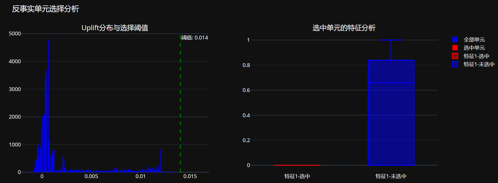
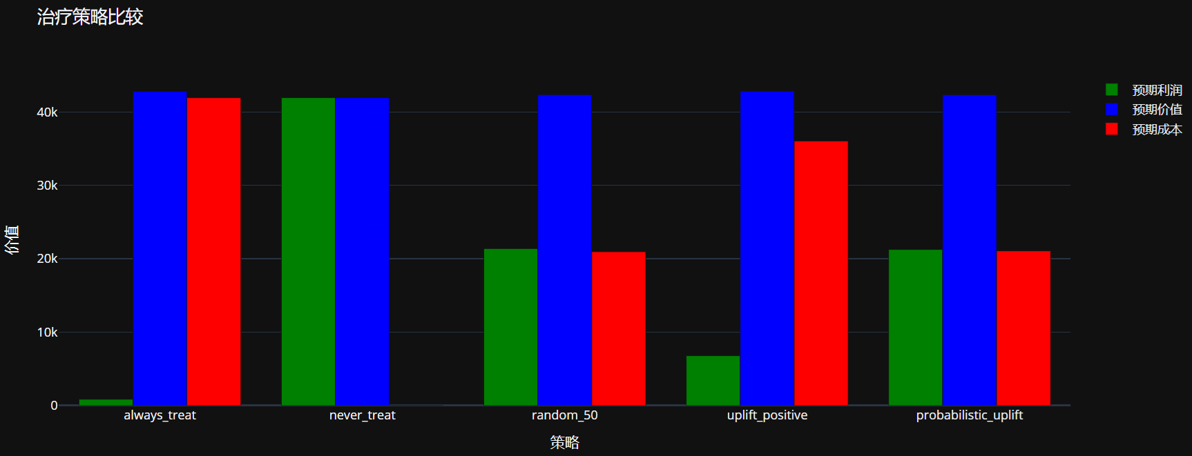
# 代码片段6.5:预算约束优化(修复版)
class BudgetConstrainedOptimizer:
    """
    预算约束优化器
    在给定预算下最大化预期价值
    """

    def __init__(self, uplift_model, treatment_cost=1.0, conversion_value=10.0):
        self.uplift_model = uplift_model
        self.treatment_cost = treatment_cost
        self.conversion_value = conversion_value
        self.optimization_results_ = None

    def optimize(self, X, budget, method='greedy'):
        """
        在预算约束下优化治疗分配

        Parameters:
        X: 特征矩阵
        budget: 预算约束
        method: 优化方法 ('greedy', 'threshold')

        Returns:
        optimization_result: 优化结果
        """
        # 预测uplift
        uplift_scores = self.uplift_model.predict(X.values) if hasattr(X, 'values') else self.uplift_model.predict(X)

        if uplift_scores.ndim > 1 and uplift_scores.shape[1] >= 2:
            uplift_scores = uplift_scores[:, 1] - uplift_scores[:, 0]
        elif uplift_scores.ndim > 1:
            uplift_scores = uplift_scores.flatten()

        n_units = len(uplift_scores)
        max_treatable = int(budget / self.treatment_cost)

        print(f"预算约束优化:")
        print(f"  总预算: {budget}")
        print(f"  治疗成本: {self.treatment_cost}")
        print(f"  最多可治疗单元数: {max_treatable}/{n_units}")

        if method == 'greedy':
            result = self._greedy_optimization(uplift_scores, max_treatable)
        elif method == 'threshold':
            result = self._threshold_optimization(uplift_scores, max_treatable)
        else:
            raise ValueError(f"未知的优化方法: {method}")

        # 计算预期价值
        expected_value = result['expected_conversions'] * self.conversion_value
        total_cost = result['n_treated'] * self.treatment_cost
        expected_profit = expected_value - total_cost

        result.update({
            'expected_value': expected_value,
            'total_cost': total_cost,
            'expected_profit': expected_profit,
            'budget_utilization': total_cost / budget
        })

        self.optimization_results_ = result

        print("优化结果:")
        for key, value in result.items():
            if isinstance(value, (int, np.integer)):
                print(f"  {key}: {value}")
            elif isinstance(value, float):
                print(f"  {key}: {value:.4f}")
            elif isinstance(value, np.ndarray):
                print(f"  {key}: [数组, 长度={len(value)}]")
            else:
                print(f"  {key}: {value}")

        return result

    def _greedy_optimization(self, uplift_scores, max_treatable):
        """贪心算法:选择uplift最高的单元"""
        # 按uplift降序排序
        sorted_indices = np.argsort(uplift_scores)[::-1]

        # 选择前max_treatable个单元
        treated_indices = sorted_indices[:max_treatable]

        # 计算预期转化数(基于平均uplift)
        avg_uplift_treated = uplift_scores[treated_indices].mean() if len(treated_indices) > 0 else 0
        baseline_conversion_rate = 0.1  # 假设基线转化率
        expected_conversions = len(treated_indices) * (baseline_conversion_rate + avg_uplift_treated)

        return {
            'n_treated': len(treated_indices),
            'treated_indices': treated_indices,
            'avg_uplift_treated': avg_uplift_treated,
            'expected_conversions': expected_conversions,
            'method': 'greedy'
        }

    def _threshold_optimization(self, uplift_scores, max_treatable):
        """阈值优化:找到最优阈值"""
        # 尝试不同的阈值
        thresholds = np.linspace(uplift_scores.min(), uplift_scores.max(), 1000)
        best_threshold = uplift_scores.min()
        best_value = 0

        for threshold in thresholds:
            # 选择高于阈值的单元
            treated_mask = uplift_scores >= threshold
            n_treated = treated_mask.sum()

            if n_treated > max_treatable:
                continue

            if n_treated == 0:
                value = 0
            else:
                avg_uplift = uplift_scores[treated_mask].mean()
                expected_conversions = n_treated * (0.1 + avg_uplift)  # 假设基线转化率10%
                value = expected_conversions * self.conversion_value - n_treated * self.treatment_cost

            if value > best_value:
                best_value = value
                best_threshold = threshold

        # 应用最佳阈值
        treated_mask = uplift_scores >= best_threshold
        treated_indices = np.where(treated_mask)[0]
        avg_uplift_treated = uplift_scores[treated_indices].mean() if len(treated_indices) > 0 else 0
        expected_conversions = len(treated_indices) * (0.1 + avg_uplift_treated)

        return {
            'n_treated': len(treated_indices),
            'treated_indices': treated_indices,
            'avg_uplift_treated': avg_uplift_treated,
            'expected_conversions': expected_conversions,
            'optimal_threshold': best_threshold,
            'method': 'threshold'
        }

    def analyze_budget_sensitivity(self, X, budget_range=None, n_points=10):
        """分析预算敏感性"""
        if budget_range is None:
            n_units = X.shape[0] if hasattr(X, 'shape') else len(X)
            max_budget = n_units * self.treatment_cost
            budget_range = np.linspace(0.1 * max_budget, max_budget, n_points)

        results = []

        for budget in budget_range:
            result = self.optimize(X, budget, method='greedy')
            results.append({
                'budget': budget,
                'expected_profit': result['expected_profit'],
                'n_treated': result['n_treated'],
                'budget_utilization': result['budget_utilization']
            })

        # 创建敏感性分析图
        budgets = [r['budget'] for r in results]
        profits = [r['expected_profit'] for r in results]
        utilizations = [r['budget_utilization'] for r in results]

        fig = make_subplots(specs=[[{"secondary_y": True}]])

        fig.add_trace(
            go.Scatter(x=budgets, y=profits, name="预期利润", line=dict(color='blue')),
            secondary_y=False
        )

        fig.add_trace(
            go.Scatter(x=budgets, y=utilizations, name="预算利用率", line=dict(color='red')),
            secondary_y=True
        )

        fig.update_layout(
            title="预算敏感性分析",
            xaxis_title="预算",
            height=500
        )

        fig.update_yaxes(title_text="预期利润", secondary_y=False)
        fig.update_yaxes(title_text="预算利用率", secondary_y=True)

        return fig, results

# 创建预算约束优化器
print("创建预算约束优化器...")
budget_optimizer = BudgetConstrainedOptimizer(
    uplift_model=best_model,
    treatment_cost=1.0,
    conversion_value=10.0
)

# 执行预算优化
budget = 5000  # 假设预算为5000
optimization_result = budget_optimizer.optimize(X_test, budget, method='greedy')

# 预算敏感性分析
sensitivity_fig, sensitivity_results = budget_optimizer.analyze_budget_sensitivity(X_test)
sensitivity_fig.show()
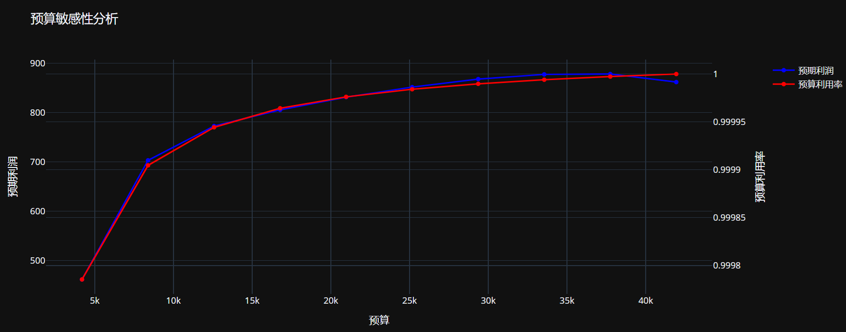
# 代码片段6.6:治疗优化综合报告
def generate_treatment_optimization_report(cus_selector, cve_estimator, budget_optimizer, X_test, W_test, Y_test):
    """生成治疗优化综合报告"""

    print("=" * 60)
    print("治疗优化综合报告")
    print("=" * 60)

    # 1. 反事实单元选择评估
    print("\n1. 反事实单元选择分析")
    print("-" * 40)

    selected_indices, uplift_scores = cus_selector.select_units(X_test)
    selection_metrics = cus_selector.evaluate_selection(X_test, W_test, Y_test, selected_indices)

    print(f"选择率: {selection_metrics['selection_rate']:.2%}")
    print(f"选中单元平均uplift: {selection_metrics.get('avg_uplift_selected', 0):.4f}")
    print(f"预期价值: {selection_metrics.get('expected_value', 0):.2f}")

    # 2. 治疗策略比较
    print("\n2. 治疗策略比较")
    print("-" * 40)

    if hasattr(cve_estimator, 'comparison_results_'):
        best_strategy = max(cve_estimator.comparison_results_.keys(),
                           key=lambda x: cve_estimator.comparison_results_[x]['expected_profit'])

        print(f"最佳策略: {best_strategy}")
        for metric, value in cve_estimator.comparison_results_[best_strategy].items():
            if isinstance(value, float):
                print(f"  {metric}: {value:.2f}")

    # 3. 预算优化结果
    print("\n3. 预算优化分析")
    print("-" * 40)

    if hasattr(budget_optimizer, 'optimization_results_'):
        result = budget_optimizer.optimization_results_
        print(f"治疗单元数: {result['n_treated']}")
        print(f"平均治疗uplift: {result.get('avg_uplift_treated', 0):.4f}")
        print(f"预期利润: {result.get('expected_profit', 0):.2f}")
        print(f"预算利用率: {result.get('budget_utilization', 0):.2%}")

    # 4. 业务建议
    print("\n4. 业务建议")
    print("-" * 40)

    # 基于分析结果提供建议
    selection_rate = selection_metrics.get('selection_rate', 0)
    expected_profit = selection_metrics.get('expected_value', 0)

    if selection_rate < 0.1:
        print("建议: 采用精准营销策略,重点关注高价值客户")
    elif selection_rate < 0.3:
        print("建议: 采用适度扩展策略,平衡覆盖面和效率")
    else:
        print("建议: 采用广泛覆盖策略,最大化市场渗透")

    if expected_profit > 0:
        print(f"预期投资回报: {expected_profit:.2f}")
        print("建议: 实施该治疗优化策略")
    else:
        print("警告: 预期利润为负,建议重新评估策略或成本结构")

    # 5. 实施注意事项
    print("\n5. 实施注意事项")
    print("-" * 40)
    print("• 定期重新训练模型以适应数据分布变化")
    print("• 监控实际效果与预测效果的差异")
    print("• 考虑实施A/B测试验证策略有效性")
    print("• 确保治疗分配系统的可靠性和公平性")

    return {
        'selection_metrics': selection_metrics,
        'strategy_comparison': getattr(cve_estimator, 'comparison_results_', {}),
        'budget_optimization': getattr(budget_optimizer, 'optimization_results_', {})
    }

# 生成综合报告
optimization_report = generate_treatment_optimization_report(
    cus_selector, cve_estimator, budget_optimizer, X_test, W_test, Y_test
)

print("\n治疗优化分析完成!")