在之前的文章中我们学习了CTR常用模型:FM、FFM和DeepFM,也学习了美团搜索广告CTR预估模型的演变。这篇文章主要从实战的角度,梳理CTR算法的使用方法。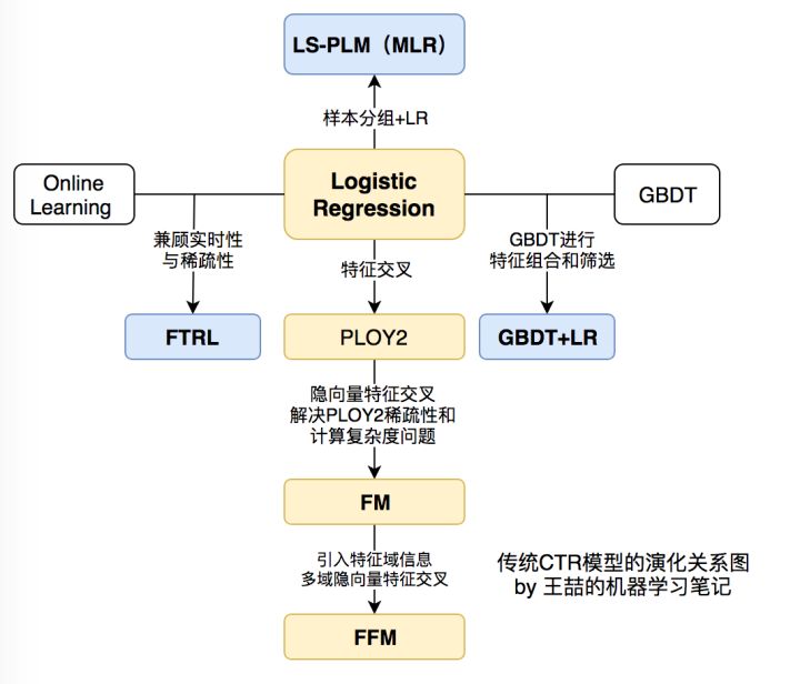
数据准备
KASANDR Data Set
Abstract: KASANDR is a novel, publicly available collection for recommendation systems that records the behavior of customers of the European leader in e-Commerce advertising, Kelkoo.
Download: Data Folder, Data Set Description
| Data Set Characteristics: | Multivariate | Number of Instances: | 17764280 | Area: | Life |
| Attribute Characteristics: | Integer | Number of Attributes: | 2158859 | Date Donated | 2017-05-16 |
| Associated Tasks: | Causal-Discovery | Missing Values? | N/A | Number of Web Hits: | 16420 |
Data Set Information:
We created this data by sampling and processing the www.kelkoo.com logs. The data records offers which were clicked (or shown) to the users of the www.kelkoo.com (and partners) in Germany as well as meta-information of these users and offers and the objective is to predict if a given user will click on a given offer.
Attribute Information:
userid offerid countrycode category merchant utcdate implicit-feedback
- csv (3,14 GB)
- Instances: 15,844,718
- Attributes: 2,299,713
- userid: Categorical, 291,485
- offerid: Categorical, 2,158,859
- countrycode: Categorical, 1 (de-Germany)
- category: Integer, 271
- merchant: Integer, 703
- utcdate: Timestamp, 2016-06-01 02:00:17.0 to 2016-06-14 23:52:51.0
- implicit feedback (click): Binary, 0 or 1
- csv (381,3 MB)
- Instances: 1,919,562
- Attributes: 2,299,713
- userid: Categorical, 278,293
- offerid: Categorical, 380,803
- countrycode: Categorical, 1
- category: Integer, 267
- merchant: Integer, 738
- utcdate: Timestamp, 2016-06-14 23:52:51.0 to 2016-07-01 01:59:36.0
- implicit feedback (click): Binary, 0 or 1
Relevant Papers:
Sumit Sidana, Charlotte Laclau, Massih-Reza Amini, Gilles Vandelle, and Andre Bois-Crettez. ‘KASANDR: A Large-Scale Dataset with Implicit Feedback for Recommendation’, SIGIR 2017.
数据说明
KASANDR这个单词,其实是Kelkoo Large Scale June Data for Recommendation的缩写,就是来源于Kelkoo这个电商网站的用户浏览记录。
数据处理
预览数据
查看数据,了解大致情况:
import pandas as pd
import numpy as np
import matplotlib.pyplot as plt

df_train = pd.read_csv('./data/de/train_de.csv', sep='\t', parse_dates=['utcdate'])
print(df_train.head())

print("The data length is %d." % (df_train.shape[0]))
features = ['userid', 'offerid', 'countrycode', 'category', 'merchant']
for feature in features:
    uniq_num = len(df_train[feature].unique())
    print("Feature %s has %d uniqure IDs." % (feature, uniq_num))

rating_count = df_train.groupby('rating').size().reset_index(name='rating_count')
print(rating_count)

user_action_count = df_train.groupby('userid').size().reset_index(name='action_count')
action_user_count = user_action_count.groupby('action_count').size().reset_index(name='user_count')
print(action_user_count.head())

item_action_count = df_train.groupby('offerid').size().reset_index(name='action_count')
action_item_count = item_action_count.groupby('action_count').size().reset_index(name='item_count')
print(action_item_count.head())

item_click_count = df_train[df_train['rating'] == 1].groupby('offerid').size().reset_index(name='click_count')
click_item_count = item_click_count.groupby('click_count').size().reset_index(name='item_count')
print(click_item_count.head())
相关字段含义为:
| 字段 | 猜测的含义 |
| userid | 用户的唯一标签 |
| offerid | 商品的唯一标签 |
| countrycode | 国家代码,由于全是Germany,所以没有什么用 |
| category | 商品分类 |
| merchant | 供应商/商家 |
| utcdate | 行为交互时间 |
| rating | 隐性行为反馈的值,0或1 |
特征准备
1、字符串特征做下encoding
from sklearn import preprocessing
for item in ['userid', 'offerid', 'category', 'merchant']:
    le = preprocessing.LabelEncoder()
    le.fit(df_train[item])
    df_train[item] = le.transform(df_train[item])
2、基于现有特征基础上增加一些聚合特征
商品热度:
| offerid_times | offerid出现次数 |
| category_times | category出现次数 |
| merchant_times | merchant出现次数 |
考虑到数字比较大,可以再使用前先进行规格化:
offerid_num_dict = df_train['offerid'].value_counts().to_dict()
category_num_dict = df_train['category'].value_counts().to_dict()
merchant_num_dict = df_train['merchant'].value_counts().to_dict()

df_train['offerid_times'] = df_train['offerid'].map(offerid_num_dict)
df_train['category_times'] = df_train['category'].map(category_num_dict)
df_train['merchant_times'] = df_train['merchant'].map(merchant_num_dict)

features_to_normalize = ['offerid_times', 'category_times', 'merchant_times']
df_train[features_to_normalize] = df_train[features_to_normalize].apply(lambda x: (x - x.min()) / (x.max() - x.min()))
df_train = df_train.rename(columns={"offerid_times": "offerid_hot", "category_times": "category_hot", "merchant_times": "merchant_hot"})
历史记录:
| pre_category | 用户产生这条记录前,产生过相同category的浏览次数 |
| pre_merchant | 用户产生这条记录前,产生过相同merchant的浏览次数 |
| pre_offerid | 用户产生这条记录前,产生过相同offerid的浏览次数 |
def find_pre(n):
    pre_dic = {}
    res = []
    for i in n.values:
        if i in pre_dic:
            res.append(pre_dic[i])
            pre_dic[i] = pre_dic[i] + 1
        else:
            res.append(0)
            pre_dic[i] = 1
    return np.array(res)

df_train['pre_category'] = df_train.groupby('userid')['category'].transform(find_pre)
df_train['pre_merchant'] = df_train.groupby('userid')['merchant'].transform(find_pre)
df_train['pre_offerid'] = df_train.groupby('userid')['offerid'].transform(find_pre)
3、去除不需要使用的特征
df_data = df_train[["userid", "offerid", "category", "merchant", "pre_offerid", "pre_category", "pre_merchant", "offerid_hot", "category_hot", "merchant_hot"]]
df_data.to_csv("./data/df.csv", index=False)
模型训练
这里使用3种方法的click预测效果,分别是LightGBM、FM和FFM。
LightGBM
代码示例:
import pandas as pd
import lightgbm as lgb
from sklearn.model_selection import GridSearchCV

df = pd.read_csv('./data/df.csv')

# 按用户抽样10%
df_train = df[df["userid"] % 10 == 0]
df_test = df[df["userid"] % 10 == 1]

X_train = df_train.iloc[:, :-1]
y_train = df_train.iloc[:, -1]
X_test = df_test.iloc[:, :-1]
y_test = df_test.iloc[:, -1]

categorical_features = ['userid', 'offerid', 'category', 'merchant']
train_data = lgb.Dataset(X_train, label=y_train)
test_data = lgb.Dataset(X_test, label=y_test, reference=train_data)

# parameters = {
# 'max_depth': [9, 11, 13],
# #'learning_rate': [0.06, 0.07],
# #'feature_fraction': [0.6, 0.65, 0.7],
# #'bagging_fraction': [0.95, 0.97, 0.99, 1],
# #'bagging_freq': [5, 6, 7, 8, 9],
# #'reg_alpha': [4, 5, 6, 7, 8],
# #'reg_lambda': [5, 6, 7, 8],
# #'cat_smooth': [0, 1, 2]
# #'num_iterations': [210, 220, 230, 240]
# }

# gbm = lgb.LGBMClassifier(objective='binary',
# is_unbalance=True,
# #metric='binary_logloss,auc',
# #max_depth=3,
# #learning_rate=0.1,
# #feature_fraction=1,
# #bagging_fraction=1,
# #bagging_freq=0,
# #reg_alpha=0,
# #reg_lambda=0,
# #cat_smooth=0,
# #num_iterations=100,
# )

# gsearch = GridSearchCV(gbm, param_grid=parameters, scoring='roc_auc', cv=3)
# gsearch.fit(X_train, y_train, categorical_feature=categorical_features)

# print('参数的最佳取值:{0}'.format(gsearch.best_params_))
# print('最佳模型得分:{0}'.format(gsearch.best_score_))
# print(gsearch.cv_results_['mean_test_score'])
# print(gsearch.cv_results_['params'])

param = {
"objective": "binary",
"is_unbalance": True,
"max_depth": 15,
"metric": ['binary_logloss', 'auc']
}
num_round = 100
bst = lgb.train(param, train_data, num_round, valid_sets=[train_data, test_data], early_stopping_rounds=10, verbose_eval=50, categorical_feature=categorical_features)
输出结果:
Training until validation scores don't improve for 10 rounds.
Early stopping, best iteration is:
[1]	training's binary_logloss: 0.152793	training's auc: 0.917826	valid_1's binary_logloss: 0.15312	valid_1's auc: 0.842001
FM
这里使用的是基于Keras的Keras的FM模型,网络结构图如下:
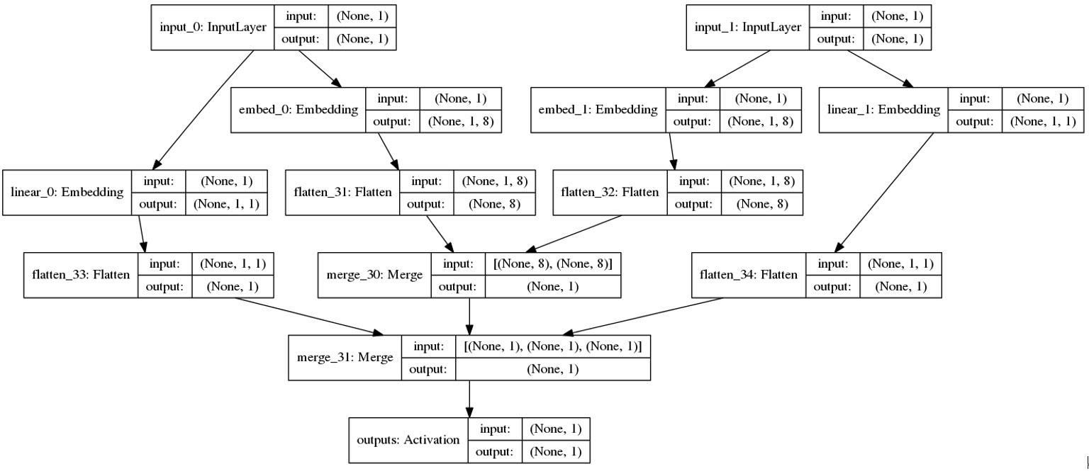
由于安装的版本不一致,这里暂未测试。
FFM
由于libffm在Windows遇到问题,所以以下代码只能在Linux环境下运行。我这里使用的是WindowsLinux子系统,安装的包:https://github.com/alexeygrigorev/libffm-python
import pandas as pd
import numpy as np
from sklearn.metrics import log_loss
from sklearn.metrics import roc_auc_score
import ffm

df = pd.read_csv('./data/df.csv')

df_train = df[df["userid"] % 10 == 0]
df_test = df[df["userid"] % 10 == 1]

X_train = df_train.iloc[:, :-1]
y_train = df_train.iloc[:, -1]
X_test = df_test.iloc[:, :-1]
y_test = df_test.iloc[:, -1]

def minmaxScale(df):
    min_data = df.min()
    max_data = df.max()
    dev_data = max_data - min_data
    return df.map(lambda x: (x - min_data) / dev_data)

def FFMDataFormat(pd_data):
    # The data format of LIBFFM is:
    # <label> <field1>:<feature1>:<value1> <field2>:<feature2>:<value2> ...
    col_list = pd_data.columns
    field_index = dict(zip(col_list, range(len(col_list))))
    base_index = 0
    for col in col_list:
        if pd_data[col].dtype == 'object':
            vals = pd_data[col].unique()
            index_dict = dict(zip(vals, range(len(vals))))
            pd_data[col] = pd_data[col].map(lambda x: (field_index[col], base_index + index_dict[x], 1))
            base_index += len(vals)
        elif pd_data[col].dtype == 'float64':
            pd_data[col] = np.round(pd_data[col], 6)
            vals = pd_data[col].unique()
            index_dict = dict(zip(vals, range(len(vals))))
            pd_data[col] = pd_data[col].map(lambda x: (field_index[col], base_index, x))
            base_index += 1
        else:
            pd_data[col] = np.round(minmaxScale(pd_data[col]), 6)
            vals = pd_data[col].unique()
            index_dict = dict(zip(vals, range(len(vals))))
            pd_data[col] = pd_data[col].map(lambda x: (field_index[col], base_index, x))
    return pd_data.values

X_train_ffm = FFMDataFormat(X_train)
y_train_ffm = y_train.tolist()

X_test_ffm = FFMDataFormat(X_test)
y_test_ffm = y_test.tolist()

ffm_train = ffm.FFMData(X_train_ffm, y_train_ffm)
ffm_test = ffm.FFMData(X_test_ffm, y_test_ffm)

n_iter = 5

ffm_model = ffm.FFM(eta=0.2, lam=0.00002, k=4)
ffm_model.init_model(ffm_train)

for i in range(n_iter):
    print('iteration %d:' % i)
    ffm_model.iteration(ffm_train)
    y_pred = ffm_model.predict(ffm_test)
    t_pred = ffm_model.predict(ffm_train)
    auc = roc_auc_score(y_test_ffm, y_pred)
    logloss = log_loss(y_test_ffm, y_pred)
    t_auc = roc_auc_score(y_train_ffm, t_pred)
    t_logloss = log_loss(y_train_ffm, t_pred)
    print('train auc %.4f, log_loss %.4f' % (t_auc, t_logloss), end='\t')
    print('test auc %.4f, log_loss %.4f' % (auc, logloss))
参考链接: