线性回归实战：波士顿房价预测

了解线性回归的原理后，为了更好的掌握相关的技能，需要进入实战，针对线性回归常见的方法有：Scikit 和 Statsmodels。

数据集的准备

美国波士顿房价的数据集是 sklearn 里面默认的数据集，sklearn 内置的数据集都位于 datasets 子模块下。一共 506 套房屋的数据，每个房屋有 13 个特征值。

from sklearn.datasets import load_boston
boston_dataset = load_boston()

print(boston_dataset.keys())
print(boston_dataset.feature_names)
print(boston_dataset.DESCR)

输出内容：

dict_keys(['data', 'target', 'feature_names', 'DESCR', 'filename'])
['CRIM' 'ZN' 'INDUS' 'CHAS' 'NOX' 'RM' 'AGE' 'DIS' 'RAD' 'TAX' 'PTRATIO'
'B' 'LSTAT'])
.. _boston_dataset:

Boston house prices dataset
---------------------------

**Data Set Characteristics:**

    :Number of Instances: 506

    :Number of Attributes: 13 numeric/categorical predictive. Median Value (attribute 14) is usually the target.

    :Attribute Information (in order):
        - CRIM     per capita crime rate by town
        - ZN       proportion of residential land zoned for lots over 25,000 sq.ft.
        - INDUS    proportion of non-retail business acres per town
        - CHAS     Charles River dummy variable (= 1 if tract bounds river; 0 otherwise)
        - NOX      nitric oxides concentration (parts per 10 million)
        - RM       average number of rooms per dwelling
        - AGE      proportion of owner-occupied units built prior to 1940
        - DIS      weighted distances to five Boston employment centres
        - RAD      index of accessibility to radial highways
        - TAX      full-value property-tax rate per $10,000
        - PTRATIO  pupil-teacher ratio by town
        - B        1000(Bk - 0.63)^2 where Bk is the proportion of black people by town
        - LSTAT    % lower status of the population
        - MEDV     Median value of owner-occupied homes in $1000's

    :Missing Attribute Values: None

    :Creator: Harrison, D. and Rubinfeld, D.L.

This is a copy of UCI ML housing dataset.
https://archive.ics.uci.edu/ml/machine-learning-databases/housing/


This dataset was taken from the StatLib library which is maintained at Carnegie Mellon University.

The Boston house-price data of Harrison, D. and Rubinfeld, D.L. 'Hedonic
prices and the demand for clean air', J. Environ. Economics & Management,
vol.5, 81-102, 1978.   Used in Belsley, Kuh & Welsch, 'Regression diagnostics
...', Wiley, 1980.   N.B. Various transformations are used in the table on
pages 244-261 of the latter.

The Boston house-price data has been used in many machine learning papers that address regression
problems.

.. topic:: References

   - Belsley, Kuh & Welsch, 'Regression diagnostics: Identifying Influential Data and Sources of Collinearity', Wiley, 1980. 244-261.
   - Quinlan,R. (1993). Combining Instance-Based and Model-Based Learning. In Proceedings on the Tenth International Conference of Machine Learning, 236-243, University of Massachusetts, Amherst. Morgan Kaufmann.

CRIM ZN INDUS CHAS NOX ... RAD TAX PTRATIO B LSTAT
0 0.00632 18.0 2.31 0.0 0.538 ... 1.0 296.0 15.3 396.90 4.98
1 0.02731 0.0 7.07 0.0 0.469 ... 2.0 242.0 17.8 396.90 9.14
2 0.02729 0.0 7.07 0.0 0.469 ... 2.0 242.0 17.8 392.83 4.03
3 0.03237 0.0 2.18 0.0 0.458 ... 3.0 222.0 18.7 394.63 2.94
4 0.06905 0.0 2.18 0.0 0.458 ... 3.0 222.0 18.7 396.90 5.33

字段解释：

• CRIM: 城镇人均犯罪率
• ZN: 住宅用地所占比例
• INDUS: 城镇中非住宅用地所占比例
• CHAS: 虚拟变量, 用于回归分析
• NOX: 环保指数
• RM: 每栋住宅的房间数
• AGE: 1940 年以前建成的自住单位的比例
• DIS: 距离 5 个波士顿的就业中心的加权距离
• RAD: 距离高速公路的便利指数
• TAX: 每一万美元的不动产税率
• PTRATIO: 城镇中的教师学生比例
• B: 城镇中的黑人比例
• LSTAT: 地区中有多少房东属于低收入人群
• MEDV: 自住房屋房价中位数（也就是均价）

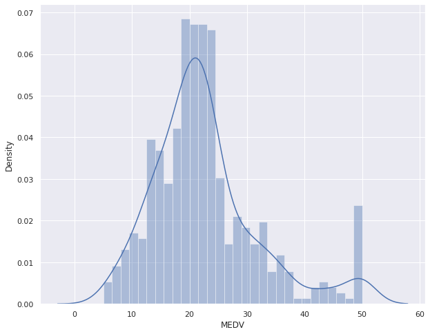
boston = pd.DataFrame(boston_dataset.data, columns=boston_dataset.feature_names)
boston['MEDV'] = boston_dataset.target

plt.figure(figsize=(10, 8))
sns.distplot(boston['MEDV'], bins=30)
plt.show()

correlation_matrix = boston.corr().round(2)
sns.heatmap(data=correlation_matrix, annot=True)
plt.show()

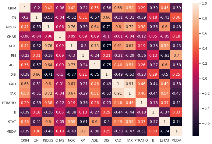
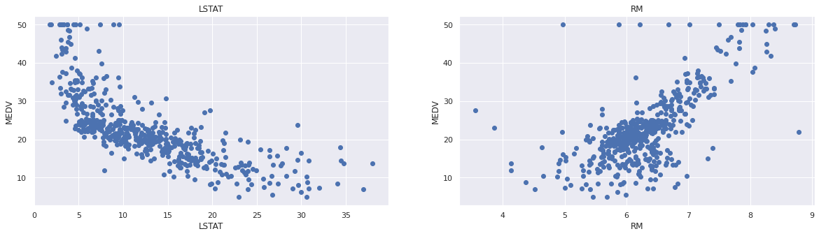
可以看到与房价相关度比较高的字段为’LSTAT’和’RM’。绘制图片，看是否存在线性关系：

plt.figure(figsize=(20, 5))

features = ['LSTAT', 'RM']
target = boston['MEDV']

for i, col in enumerate(features):
    plt.subplot(1, len(features), i+1)
    x = boston[col]
    y = target
    plt.scatter(x, y, marker='o')
    plt.title(col)
    plt.xlabel(col)
    plt.ylabel('MEDV')

数据准备：

from sklearn.model_selection import train_test_split

X = boston[['LSTAT', 'RM']]
y = boston['MEDV']
X_train, X_test, y_train, y_test = train_test_split(X, y, test_size=0.2, random_state=5)

sklearn.linear_model.LinearRegression

示例代码：

import pandas as pd
import numpy as np
from sklearn.model_selection import train_test_split
from sklearn.linear_model import LinearRegression
from sklearn.metrics import mean_squared_error
from sklearn.metrics import r2_score

from sklearn.datasets import load_boston

boston_dataset = load_boston()

boston = pd.DataFrame(boston_dataset.data, columns=boston_dataset.feature_names)
boston['MEDV'] = boston_dataset.target

X = boston[['LSTAT', 'RM']]
y = boston['MEDV']
X_train, X_test, y_train, y_test = train_test_split(X, y, test_size=0.2, random_state=5)

lr = LinearRegression()
lr.fit(X_train, y_train)
#打印截距
print(lr.intercept_)
#打印模型系数
print(lr.coef_)
y_test_predict = lr.predict(X_test)

rmse = np.sqrt(mean_squared_error(y_test, y_test_predict))
r2 = r2_score(y_test, y_test_predict)
print(rmse, r2)

StatsModels OLS

Statsmodels的OSL是回归模型中最常用的最小二乘法求解法。

import pandas as pd
from sklearn.datasets import load_boston
from sklearn.model_selection import train_test_split
import statsmodels.api as sm

boston_dataset = load_boston()

boston = pd.DataFrame(boston_dataset.data, columns=boston_dataset.feature_names)
boston['MEDV'] = boston_dataset.target

X = boston[['LSTAT', 'RM']]
y = boston['MEDV']
X_train, X_test, y_train, y_test = train_test_split(X, y, test_size=0.2, random_state=5)

result = sm.OLS(y_train, X_train).fit()
print(result.params)
print(result.summary())

这里需要重要介绍的是如何读懂报告。

OLS Regression Results
=======================================================================================
Dep. Variable: MEDV R-squared (uncentered): 0.947
Model: OLS Adj. R-squared (uncentered): 0.947
Method: Least Squares F-statistic: 3581.
Date: Fri, 06 Aug 2021 Prob (F-statistic): 6.67e-257
Time: 16:07:31 Log-Likelihood: -1272.2
No. Observations: 404 AIC: 2548.
Df Residuals: 402 BIC: 2556.
Df Model: 2
Covariance Type: nonrobust
==============================================================================
 coef std err t P>|t| [0.025 0.975]
------------------------------------------------------------------------------
LSTAT -0.6911 0.036 -19.367 0.000 -0.761 -0.621
RM 4.9699 0.081 61.521 0.000 4.811 5.129
==============================================================================
Omnibus: 121.894 Durbin-Watson: 2.063
Prob(Omnibus): 0.000 Jarque-Bera (JB): 389.671
Skew: 1.370 Prob(JB): 2.42e-85
Kurtosis: 6.954 Cond. No. 4.70
==============================================================================

Notes:
[1] R² is computed without centering (uncentered) since the model does not contain a constant.
[2] Standard Errors assume that the covariance matrix of the errors is correctly specified.

如何解读报告？来看一些名词解释：

• Variable: 就是因变量，dependent variable，也就是输入的y的名称。
• Model：这里就是OLS。
• Method：使用最小二乘法的方法确定参数
• Date：模型生成的日期。
• Time：模型生成的具体时间。
• Observations：样本量，就是输入的数据量。
• Df Residuals：残差自由度，即degree of freedom of residuals。
• DfModel：模型自由度，degree of freedom of model，模型参数个数（不包含常量参数），对应于 coef 中的行数
• CovarianceType：协方差类型。
• R-squared：可决系数，说明估计的准确性。“可决系数”是通过数据的变化来表征一个拟合的好坏。其值=SSR/SST，SSR 是 Sum of Squares for Regression，SST 是 Sum of Squares for Total，这个值范围在[0,1]，其值越接近1，说明回归效果越好。
• R-squared：利用奥卡姆剃刀原理，对 R-squared 进行修正。公式$R_{adj}^2=1-\frac{(n-1)(1-R^2}{n-p-1}$。其中 n 是样本数量(No. Observations)，p 是模型中变量的个数(Df Model)。
• F-statistic：统计检验 F 统计量，值越大越能推翻原假设（原假设是“模型不是线性模型”），所以值过大，说明我们的模型是线性模型。F=Model Mean Square/Error Mean Square
• Prob(F-statistic)：F 检验的 P 值，这个值越小越能拒绝原假设，值越小越证明模型是线性显著的。
• Log likelihood：对数似然。对数函数和似然函数具有同一个最大值点。取对数是为了方便计算极大似然估计，通常先取对数再求导，找到极值点。这个参数很少使用，可以不考虑。
• AIC：其用来衡量拟合的好坏程度，一般选择 AIC 较小的模型。
• BIC：贝叶斯信息准则，其比 AIC 在大数据量时，对模型参数惩罚得更多，所以 BIC 更倾向于选择参数少的简单模型。
• coef：指自变量和常数项的系数
• stderr：系数估计的标准误差。
• t：就是我们常用的 t 统计量，这个值越大越能拒绝原假设。
• P>|t|：统计检验中的 P 值，这个值越小越能拒绝原假设。
• [0.025,0.975]：这个是置信度为95%的置信区间的下限和上限。
• Omnibus：基于峰度和偏度进行数据正态性的检验，其常和 Jarque-Bera 检验一起使用。
• Prob(Omnibus)：基于峰度和偏度进行数据正态性的检验概率
• Durbin-Watson：检验残差中是否存在自相关，其主要通过确定两个相邻误差项的相关性是否为零来检验回归残差是否存在自相关。
• Skewness：偏度，反映数据分布的非对称程度
• Kurtosis：峰度，反映数据分布陡峭或平滑程度
• Jarque-Bera(JB)：基于峰度和偏度对数据正态性的检验
• Prob(JB)：Jarque-Bera(JB)检验的 P 值
• No.：多重共线性的检验，即检验变量之间是否存在精确相关关系或高度相关关系。