Optuna 超参数优化从入门到实战
超参数优化(Hyperparameter Optimization, HPO)是机器学习流程中最耗时也最关键的一环。手动调参靠直觉、网格搜索靠暴力、随机搜索靠运气——而 Optuna 提供了一种更聪明的方式:让优化器从历史 Trial 中学习,自适应地聚焦到高潜力参数区域。
Optuna 由 Preferred Networks 开发,是当前最流行的 Python 超参数优化框架之一。先看看传统超参数优化方案的痛点:
| 方案 | 原理 | 优点 | 缺点 |
| 手动调参 | 凭经验逐个尝试 | 灵活、可结合先验 | 不可复现,效率极低 |
| Grid Search | 穷举所有参数组合 | 覆盖全面 | 维度灾难,指数增长 |
| Random Search | 随机采样参数 | 实现简单、无偏 | 不利用历史,资源浪费 |
| Bayesian (TPE) | 基于历史建模采样 | 自适应、高效 | 需要足够的启动 Trial |
Optuna 的核心优势在于:
- Define-by-Run:搜索空间在 objective 函数内动态定义,支持条件参数、动态搜索空间
- 自适应采样:默认使用 TPE(Tree-structured Parzen Estimator),从历史 Trial 中学习并聚焦高潜力区域
- 剪枝机制:提前终止表现不佳的 Trial,大幅节省计算资源
- 可视化:内置 8 种可视化图表 + Dashboard 实时监控
- 分布式:支持多进程/多机并行优化,存储后端可替换(SQLite/Redis/MySQL)
- 生态集成:与 LightGBM、XGBoost、PyTorch、TensorFlow、sklearn 等无缝集成
Optuna的核心架构
Optuna 的架构围绕五个核心概念展开:Study、Trial、Objective、Sampler 和 Pruner。 理解它们的关系是掌握 Optuna 的基础。
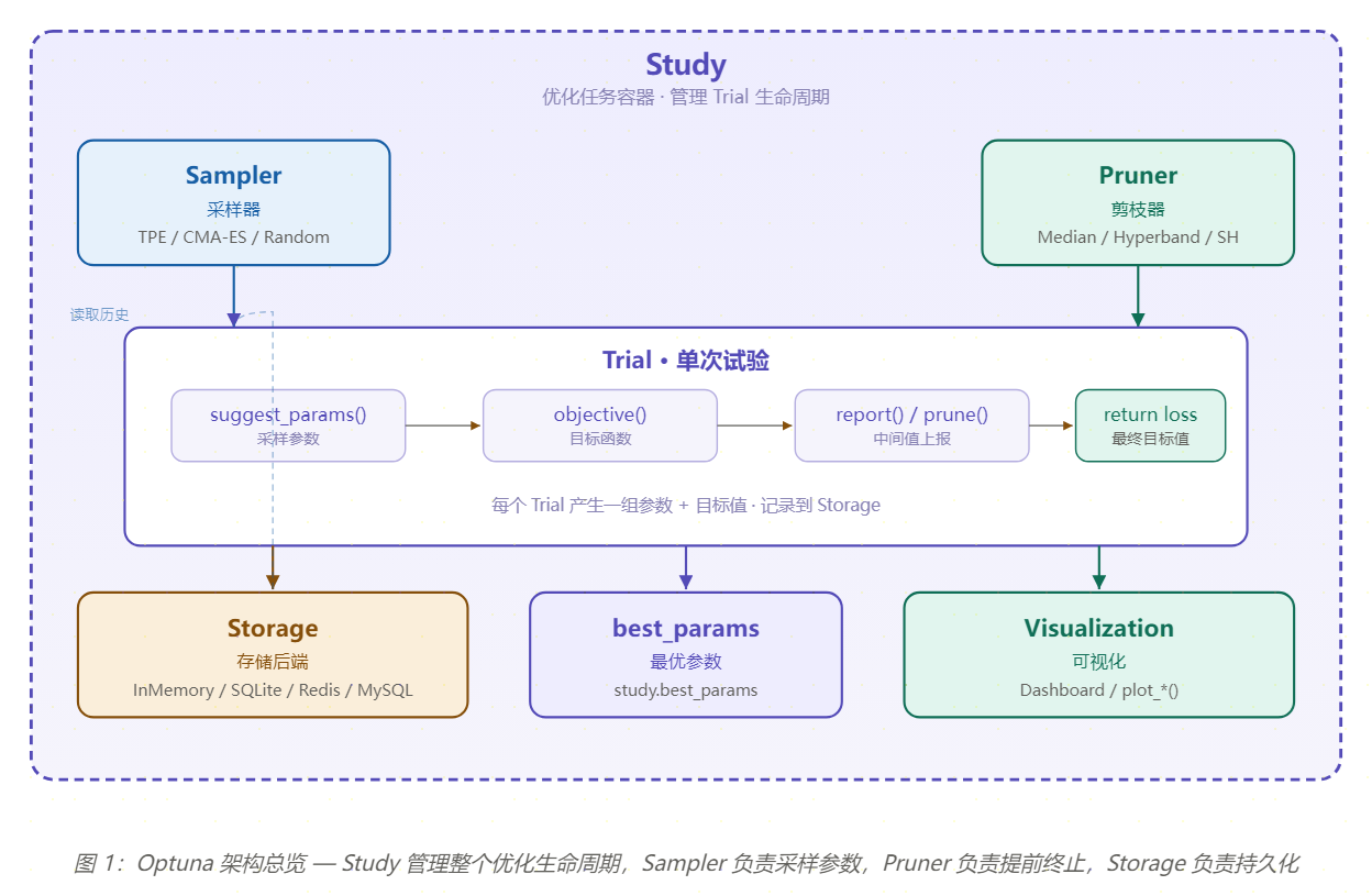
各组件的职责:
| 组件 | 角色 | 关键属性/方法 |
| Study | 优化任务容器,管理所有 Trial | direction · sampler · pruner · best_params |
| Trial | 单次参数试验 | suggest_*() · report() · should_prune() |
| Objective | 用户定义的目标函数 | 输入 trial,输出 loss(float) |
| Sampler | 参数采样策略 | TPE / CMA-ES / Random / Grid |
| Pruner | 提前终止策略 | Median / SuccessiveHalving / Hyperband |
| Storage | 持久化后端 | InMemory / SQLite / Redis / MySQL |
优化循环的工作流程:
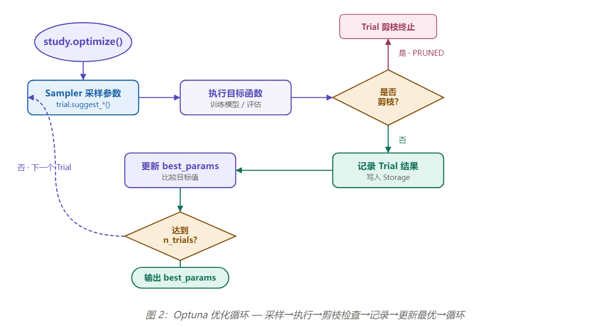
核心流程解读:
- optimize()启动优化循环
- Sampler根据历史 Trial 分布,为当前 Trial 建议一组参数(suggest_*())
- 执行Objective 函数:用建议的参数训练模型并评估
- 训练过程中可以调用report(loss, step) 上报中间值
- Pruner判断当前 Trial 是否值得继续:如果表现不佳 → TrialPruned() 提前终止
- 完成的 Trial 结果写入Storage,更新 best_params
- 循环直到达到n_trials 或 timeout
快速上手:5 分钟入门
安装
# 基础安装
pip install optuna

# 带可视化扩展
pip install optuna[visualization]

# 完整安装(含所有可选依赖)
pip install optuna[all]
第一个示例
Optuna 的核心就三步:定义 objective(在函数内用 trial.suggest_*() 声明参数和范围)→ 创建 Study(指定优化方向 minimize/maximize)→ 启动优化(study.optimize())。
import optuna

def objective(trial):
    # 定义搜索空间
    lr = trial.suggest_float("lr", 1e-5, 1e-1, log=True)
    n_layers = trial.suggest_int("n_layers", 2, 8)
    dropout = trial.suggest_float("dropout", 0.0, 0.5)
    hidden_dim = trial.suggest_categorical("hidden_dim", [32, 64, 128, 256])
    optimizer_name = trial.suggest_categorical("optimizer", ["Adam", "SGD", "RMSprop"])

    # 用建议的参数训练模型(这里用模拟值演示)
    # 实际场景中替换为你的训练 + 验证逻辑
    loss = (lr * 10 + n_layers * 0.1 + dropout * 2
            + (1 if optimizer_name == "Adam" else 0.5)
            + (256 - hidden_dim) * 0.001)

    return loss  # 返回需要最小化的目标值

# 创建 Study 并优化
study = optuna.create_study(direction="minimize")
study.optimize(objective, n_trials=50)

# 查看结果
print(f"最佳目标值: {study.best_value:.6f}")
print(f"最佳参数: {study.best_params}")
运行后输出类似:
[I 2026-08-18 10:30:12,123] Trial 0 finished with value: 0.512345 and parameters: {'lr': 0.0234, 'n_layers': 4, ...}. Best is trial 0 with value: 0.512345.
...
[I 2026-08-18 10:31:45,678] Trial 49 finished with value: 0.000123 and parameters: {'lr': 0.00156, 'n_layers': 3, ...}. Best is trial 49.
最佳目标值: 0.788568
最佳参数: {'lr': 8.384804183578591e-05, 'n_layers': 2, 'dropout': 0.043864761654720225, 'hidden_dim': 256, 'optimizer': 'RMSprop'}
运行后,你会看到每个 Trial 的日志输出,最终得到最佳目标值和对应的参数组合。整个过程无需手动管理搜索空间——参数的声明和采样都在 objective 函数内部完成,这就是 Define-by-Run 的核心优势。
suggest 方法速查
| 方法 | 用途 | 示例 | 适用场景 |
| suggest_float | 浮点数 | suggest_float(‘lr’, 1e-5, 1e-1, log=True) | 学习率(对数尺度) |
| suggest_int | 整数 | suggest_int(‘n_layers’, 2, 8) | 层数、树数量 |
| suggest_categorical | 分类 | suggest_categorical(‘opt’, [‘Adam’,’SGD’]) | 优化器类型、离散选择 |
| suggest_float(log=True) | 对数浮点 | suggest_float(‘reg’, 1e-8, 10, log=True) | 正则化系数 |
| suggest_discrete_uniform | 离散均匀 | suggest_discrete_uniform(‘drop’, 0, 0.5, 0.1) | 步长固定的连续值 |
对于学习率、正则化系数等跨多个数量级的参数,log=True 让采样器在对数空间均匀采样。例如 suggest_float(‘lr’, 1e-5, 1e-1, log=True) 会在 [0.00001, 0.0001, 0.001, 0.01, 0.1] 之间均匀分布,而非在 [0, 0.1] 线性空间中偏向大值。这是初学者最常犯的错误之一。
采样器与采样策略
Sampler 决定了 Optuna 如何从历史 Trial 中学习并建议下一组参数。选择合适的 Sampler 是优化效率的关键。
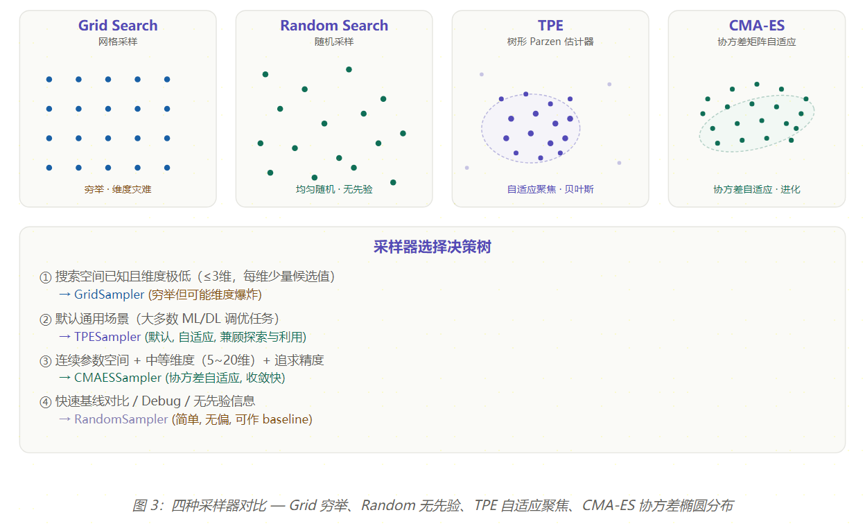
TPE(Tree-structured Parzen Estimator)
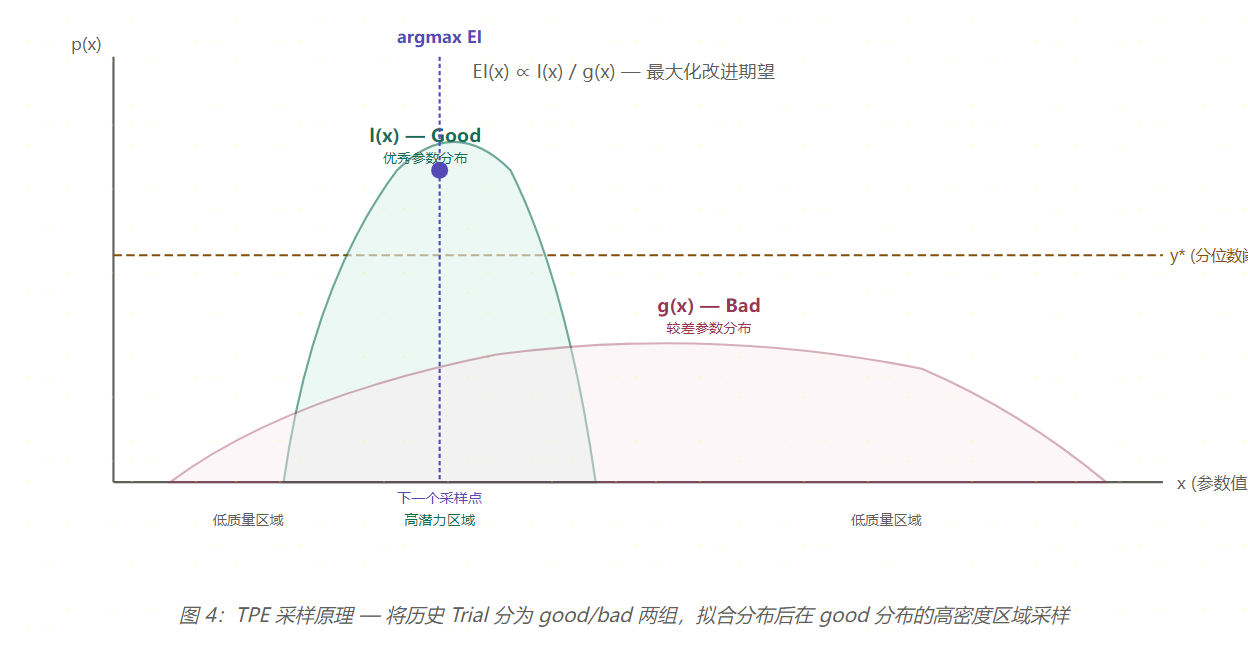
TPE 是 Optuna 的默认采样器,也是大多数场景的推荐选择。它的核心思想是:
- 将历史 Trial 按目标值分为两组:good(低于分位数阈值 y*)和bad(高于 y*)
- 分别拟合两个分布:l(x)(good 分布)和g(x)(bad 分布)
- 计算 Expected Improvement:EI(x) ∝ l(x) / g(x)
- 从l(x) 中采样,选择使 EI 最大的参数
TPE 的关键参数
- n_startup_trials(默认 10):启动阶段的随机采样次数。在收集足够历史数据前,TPE 退化为随机搜索。
- multivariate=True(推荐开启):多变量联合建模,捕获参数间的相关性,显著提升优化效率。
- n_ei_candidates(默认 24):EI 候选数量,越大越精细但每次采样更慢。
CMA-ES(协方差矩阵自适应进化策略)
CMA-ES 是一种进化策略算法,通过自适应调整协方差矩阵来引导搜索方向。它特别适合:
- 连续参数空间
- 中等维度(5~20 维)
- 参数间存在非线性交互
- 追求高精度收敛
CMA-ES 的核心机制是维护一个多元高斯分布 N(m, σ²C),其中 C 是协方差矩阵, 随着迭代自适应更新,让搜索椭圆自动对齐到目标函数的地形方向。
采样器选择指南
| 采样器 | 维度适用 | 参数类型 | 优势 | 推荐场景 |
| TPE | 任意 | 混合(连续+离散) | 自适应、稳定、支持条件参数 | 默认推荐 大多数 ML/DL |
| CMA-ES | 5~20 | 连续 | 高精度收敛 | 深度调优连续参数 |
| Random | 任意 | 任意 | 无偏、快速 | 基线对比 / Debug |
| Grid | ≤3 | 离散 | 穷举无遗漏 | 低维精确搜索 |
import optuna

# ─── TPE 采样器(默认,推荐大多数场景)──
sampler_tpe = optuna.samplers.TPESampler(
    n_startup_trials=10,   # 前 10 次随机采样(建立先验)
    n_ei_candidates=24,    # EI 候选数,越大越精细但越慢
    multivariate=True,     # 多变量联合建模(推荐开启)
    seed=42,               # 固定随机种子
)

# ─── CMA-ES 采样器(适合连续参数 + 中等维度)──
sampler_cmaes = optuna.samplers.CMAESampler(
    n_startup_trials=10,   # 启动阶段用随机采样
    sigma=0.3,             # 初始步长(搜索范围的比例)
    seed=42,
)

# ─── 随机采样器(基线对比 / Debug)──
sampler_random = optuna.samplers.RandomSampler(seed=42)

# ─── 网格采样器(低维穷举)──
sampler_grid = optuna.samplers.GridSampler(
    search_space={
        "lr": [1e-5, 1e-4, 1e-3, 1e-2, 1e-1],
        "batch_size": [32, 64, 128, 256],
    }
)

# 使用采样器创建 Study
study = optuna.create_study(
    direction="minimize",
    sampler=sampler_tpe,
    study_name="my_experiment",
    storage="sqlite:///example.db",  # 持久化存储
)
study.optimize(objective, n_trials=100)
剪枝器:提前终止无效试验
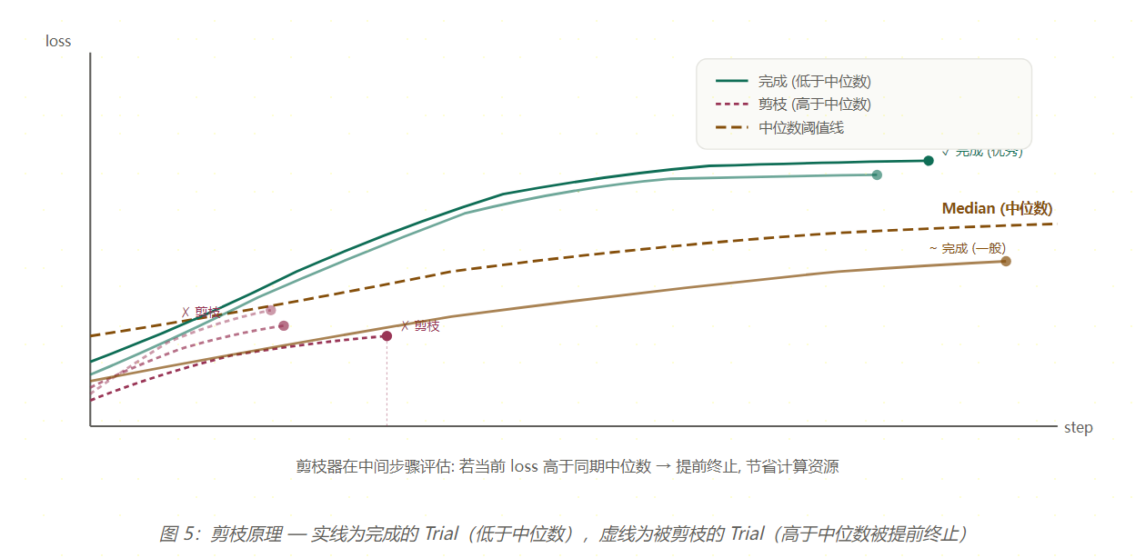
剪枝(Pruning)是 Optuna 最强大的功能之一。在深度学习训练中,一个 Trial 可能需要跑 100 个 epoch, 但如果第 10 个 epoch 的 loss 已经远高于中位数,继续跑下去基本是浪费时间。 剪枝器可以在训练过程中实时判断,提前终止没有前途的 Trial。
三种剪枝器对比
| 剪枝器 | 核心思想 | 优势 | 适用场景 |
| MedianPruner | 当前 loss 高于同期中位数则剪枝 | 简单、稳定 | 通用基线 |
| SuccessiveHalving | 逐步淘汰表现差的配置 | 资源分配高效 | 已知最大资源步数 |
| HyperbandPruner | 多组不同资源配置并行淘汰 | 自动平衡探索/利用 | 推荐 深度学习 |
使用示例:
import optuna

# ─── MedianPruner(默认,简单高效)──
pruner_median = optuna.pruners.MedianPruner(
    n_startup_trials=5,       # 前 5 个 Trial 不剪枝
    n_warmup_steps=10,       # 每个 Trial 前 10 步不剪枝
    interval_steps=1,        # 每步都检查
)

# ─── SuccessiveHalvingPruner(SHA)──
pruner_sha = optuna.pruners.SuccessiveHalvingPruner(
    min_resource=1,           # 最少资源单位
    reduction_factor=4,      # 每轮淘汰 3/4
    min_early_stopping_rate=0,
)

# ─── HyperbandPruner(推荐,多保真优化)──
pruner_hyperband = optuna.pruners.HyperbandPruner(
    min_resource=1,
    max_resource=100,         # 最大资源(epoch 数)
    reduction_factor=3,
)

# ─── NopPruner(不剪枝,作为基线)──
pruner_nop = optuna.pruners.NopPruner()

# 在 objective 中配合使用
def objective_with_pruning(trial):
    model = build_model(trial.params)

    for epoch in range(100):
        loss = train_one_epoch(model, epoch)

        # 上报中间值 → 剪枝器判断是否提前终止
        trial.report(loss, epoch)

        if trial.should_prune():
            raise optuna.TrialPruned()  # 主动剪枝

    return loss  # 最终目标值

study = optuna.create_study(
    direction="minimize",
    pruner=pruner_hyperband,
)
study.optimize(objective_with_pruning, n_trials=200)
剪枝的常见误区:
- 误区 1:剪枝器设得太激进。n_warmup_steps设为 0 会导致前几步 loss 还在波动时就剪枝, 误杀很多有潜力的 Trial。建议 n_warmup_steps 至少为总步数的 10%。
- 误区 2:忘了在 objective 中调用should_prune()。剪枝器需要 trial.report() 上报中间值才能工作。
- 误区 3:上报的中间值方向不一致。如果direction=”minimize”,中间值也应该是”越小越好”的指标。
搜索空间设计方法论
搜索空间的设计直接影响优化效率——好的搜索空间能让 100 个 Trial 达到差的搜索空间 1000 个 Trial 的效果。搜索空间设计之所以难,核心原因只有一个:维度灾难(Curse of Dimensionality)。每增加一个参数,搜索空间的体积呈指数增长,采样器需要更多的 Trial 才能覆盖。
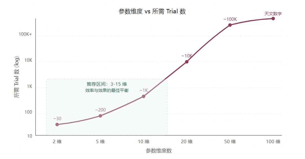
如上所示,2 维只需约 30 个 Trial 就能找到不错的结果,但到了 20 维就需要 10000+ 个 Trial。这就是为什么减少不必要的参数维度是搜索空间设计的头等大事。
减少维度:三个核心策略
搜索空间维度是效率的第一杀手。以下三个策略可以把维度从 30+ 降到 10 以内:
- 策略 1:固定不重要参数。不是所有参数都值得搜索。先用少量 Trial 跑一轮,看 plot_param_importances,重要性 < 5% 的参数直接固定为默认值。
- 策略 2:条件参数。只在需要时才 suggest 参数——避免搜索空间组合爆炸。
- 策略 3:参数共享。多层网络不要每层独立搜索,用一组共享参数控制所有层。
# 反面:每层独立参数 → 10 层就是 30 维
def objective_bad(trial):
    n_layers = trial.suggest_int("n_layers", 1, 10)
    for i in range(n_layers):
        trial.suggest_float(f"lr_{i}", 1e-5, 1e-1, log=True)     # 10 维
        trial.suggest_int(f"units_{i}", 16, 512)                   # 10 维
        trial.suggest_float(f"dropout_{i}", 0, 0.5)                # 10 维
    # 总计 31 维 → 需要 10K+ trials
    return train_model(...)

# 正确:共享参数 + 条件参数 → 总共 5 维
def objective_good(trial):
    n_layers = trial.suggest_int("n_layers", 1, 6)
    hidden_dim = trial.suggest_categorical("hidden_dim", [64, 128, 256])
    dropout = trial.suggest_float("dropout", 0.0, 0.5)
    lr = trial.suggest_float("lr", 1e-5, 1e-1, log=True)
    weight_decay = trial.suggest_float("wd", 1e-6, 1e-2, log=True)
    # 条件参数:只有层数多时才搜 extra regularization
    if n_layers > 4:
        extra_l2 = trial.suggest_float("extra_l2", 1e-6, 1e-2, log=True)
    else:
        extra_l2 = 0.0  # 不进入搜索空间
    return train_model(n_layers, hidden_dim, dropout, lr, weight_decay, extra_l2)
    # 总计 5~6 维 → 200 trials 足够
两阶段搜索法:先粗后精
这是实战中最有效的策略:不要一上来就在大范围里跑 1000 个 Trial,而是分两轮。Phase 1 用宽范围跑 50 个 Trial,分析参数重要性和最优区间;Phase 2 缩小范围到高潜力区域,固定不重要的参数,跑 100 个 Trial 精细搜索。总计 150 个 Trial,效果优于单轮 500 个 Trial。
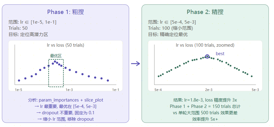
两阶段搜索的代码实现也相当简洁,关键是在 Phase 1 结束后用 plot_param_importances 和 plot_slice 分析结果,然后为 Phase 2 重新创建一个缩小范围的 Study:
import optuna

# ─── Phase 1: 粗搜(宽范围,少 trials)──
def objective_phase1(trial):
    lr = trial.suggest_float("lr", 1e-5, 1e-1, log=True)
    n_layers = trial.suggest_int("n_layers", 1, 8)
    dropout = trial.suggest_float("dropout", 0.0, 0.5)
    hidden_dim = trial.suggest_categorical("hidden_dim", [32, 64, 128, 256])
    weight_decay = trial.suggest_float("wd", 1e-8, 1.0, log=True)
    return train_and_evaluate(lr, n_layers, dropout, hidden_dim, weight_decay)

study1 = optuna.create_study(direction="minimize",
    sampler=optuna.samplers.TPESampler(seed=42),
    storage="sqlite:///phase1.db")
study1.optimize(objective_phase1, n_trials=50)

# 分析 Phase 1 结果
importances = optuna.importance.get_param_importances(study1)
# 假设结果: lr=65%, n_layers=20%, hidden_dim=8%, wd=5%, dropout=2%
# → dropout 几乎没影响,固定为 0.1
# → lr 最重要,看 slice plot 发现最优在 [5e-4, 5e-3]

# ─── Phase 2: 精搜(缩小范围,更多 trials)──
def objective_phase2(trial):
    lr = trial.suggest_float("lr", 5e-4, 5e-3, log=True)
    dropout = 0.1               # 固定(Phase 1 显示不重要)
    n_layers = trial.suggest_int("n_layers", 3, 6)
    hidden_dim = 128            # 固定(Phase 1 最优)
    weight_decay = trial.suggest_float("wd", 1e-6, 1e-3, log=True)
    return train_and_evaluate(lr, n_layers, dropout, hidden_dim, weight_decay)

study2 = optuna.create_study(direction="minimize",
    sampler=optuna.samplers.TPESampler(seed=42),
    storage="sqlite:///phase2.db")
study2.optimize(objective_phase2, n_trials=100)
参数设计速查表
| 参数 | 类型 | 推荐范围 | log=True? | 理由 |
| learning_rate | float | [1e-5, 1e-1] | 是 | 跨 4 个数量级 |
| weight_decay | float | [1e-8, 1e-2] | 是 | 跨 6 个数量级 |
| dropout | float | [0.0, 0.5] | 否 | 同量级,比值 0.5 |
| batch_size | categorical | [32, 64, 128, 256] | N/A | 离散选择,2 的幂 |
| n_layers | int | [1, 6] | 否 | 小范围整数 |
| hidden_dim | categorical | [64, 128, 256, 512] | N/A | 离散选择 |
| num_leaves (LGB) | int | [15, 255] | 是 | 大范围,log 更均匀 |
| subsample | float | [0.5, 1.0] | 否 | 同量级 |
| colsample_bytree | float | [0.5, 1.0] | 否 | 同量级 |
| reg_alpha | float | [1e-8, 10.0] | 是 | 跨 9 个数量级 |
| reg_lambda | float | [1e-8, 10.0] | 是 | 跨 9 个数量级 |
| momentum | float | [0.5, 0.99] | 否 | 同量级 |
| label_smoothing | float | [0.0, 0.2] | 否 | 同量级 |
判断规则很简单:看 min/max 的比值。如果比值大于 100(比如 1e-5 到 1e-1 的比值是 10000),就该用 log=True。
可视化分析
Optuna 内置了 8 种可视化图表,所有图表都基于 Plotly,支持交互式查看 ,配合 Dashboard 可以实时监控优化进度。这是 Optuna 相比其他 HPO 框架的一大优势——不用自己写绘图代码。
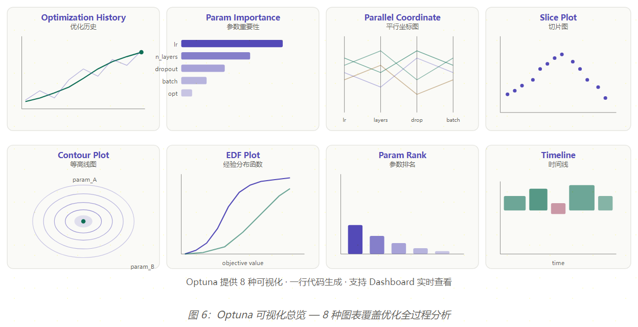
八种可视化图表
| 图表 | 函数 | 核心用途 | 何时使用 |
| Optimization History | plot_optimization_history | 目标值随 Trial 的变化趋势 | 查看收敛速度 |
| Param Importance | plot_param_importances | 各参数对目标值的贡献度 | 识别关键超参 |
| Parallel Coordinate | plot_parallel_coordinate | 多参数联合分布可视化 | 发现好的参数组合 |
| Slice Plot | plot_slice | 单参数 vs 目标值散点 | 定位参数最优区间 |
| Contour Plot | plot_contour | 双参数交互的等高线 | 分析参数交互 |
| EDF | plot_edf | 目标值的经验分布函数 | 对比多个 Study |
| Param Rank | plot_rank | 参数排名分布 | 查看参数稳定性 |
| Timeline | plot_timeline | Trial 执行时间线 | 分析耗时瓶颈 |
import optuna

# 假设 study 已优化完毕
# study = optuna.create_study(direction="minimize")
# study.optimize(objective, n_trials=100)

# ─── 1. 优化历史 ──
fig = optuna.visualization.plot_optimization_history(study)
fig.show()  # 或 fig.write_html("optimization_history.html")

# ─── 2. 参数重要性 ──
fig = optuna.visualization.plot_param_importances(study)
fig.show()

# ─── 3. 平行坐标图(查看参数组合)──
fig = optuna.visualization.plot_parallel_coordinate(study)
fig.show()

# ─── 4. 切片图(单参数 vs 目标值)──
fig = optuna.visualization.plot_slice(study, params=["lr", "n_layers"])
fig.show()

# ─── 5. 等高线图(双参数交互)──
fig = optuna.visualization.plot_contour(study, params=["lr", "dropout"])
fig.show()

# ─── 6. 经验分布函数 ──
fig = optuna.visualization.plot_edf(study)
fig.show()

# ─── 7. 参数关系图 ──
fig = optuna.visualization.plot_rank(study)
fig.show()

# ─── 8. 时间线(查看 Trial 执行顺序和耗时)──
fig = optuna.visualization.plot_timeline(study)
fig.show()

# ─── 启动 Dashboard(实时监控)──
# 终端运行: optuna-dashboard sqlite:///example.db  ./dashboard
# 或 Python 内启动:
# from optuna_dashboard import run_server
# run_server("sqlite:///example.db")
Dashboard 实时监控
对于长时间运行的优化任务,推荐使用 Optuna Dashboard 实时查看优化进度:
pip install optuna-dashboard
optuna-dashboard sqlite:///example.db ./dashboard
Dashboard 会自动刷新,无需中断优化即可查看所有图表和 Trial 详情。
实战常见问题与解决方案
以下是在实际项目中反复出现的问题,按严重程度排列。
问题 1:Objective 返回 NaN / Inf
某些参数组合下,模型训练可能产生 NaN(如学习率过大导致梯度爆炸)。如果不处理,Study 会崩溃或产生无效结果。正确做法是在 objective 中添加检查,遇到异常值时 raise TrialPruned() 或返回一个较大的惩罚值。
# 错误:objective 可能返回 NaN
def objective_bad(trial):
    lr = trial.suggest_float("lr", 0, 1)
    # 某些参数组合下可能产生 NaN
    loss = some_unstable_computation(lr)
    return loss  # NaN 会导致 Study 崩溃

# 正确:添加 NaN/Inf 检查
def objective_safe(trial):
    lr = trial.suggest_float("lr", 1e-5, 1e-1, log=True)
    loss = some_computation(lr)

    # 检查异常值
    if not np.isfinite(loss):
        raise optuna.TrialPruned()  # 或返回一个较大的惩罚值
        # return float("inf")  # 替代方案:返回大值

    return loss
问题 2:搜索空间设计不合理
搜索空间过大或维度过高是优化效率低下的最主要原因。条件参数未正确处理会导致搜索空间组合爆炸。核心对策是使用共享参数代替每层独立参数,用 if 条件减少不必要的参数维度——将 30+ 维降到 10 维以内。
# 错误:无条件建议所有参数 → 搜索空间爆炸
def objective_bad(trial):
    n_layers = trial.suggest_int("n_layers", 1, 10)
    # 每层都有独立参数 → 组合爆炸
    for i in range(n_layers):
        trial.suggest_float(f"lr_{i}", 1e-5, 1e-1, log=True)
        trial.suggest_int(f"units_{i}", 16, 256)
    return train_model(...)

#正确:使用条件参数空间
def objective_good(trial):
    n_layers = trial.suggest_int("n_layers", 1, 5)
    hidden_dim = trial.suggest_categorical("hidden_dim", [64, 128, 256])
    dropout = trial.suggest_float("dropout", 0.0, 0.5)

    # 共享参数而非每层独立 → 减少维度
    # 只在需要时建议额外参数
    if n_layers > 3:
        extra_reg = trial.suggest_float("extra_l2", 1e-6, 1e-2, log=True)
    else:
        extra_reg = 0.0

    return train_model(n_layers, hidden_dim, dropout, extra_reg)
问题 3:剪枝过于激进
n_warmup_steps 设置过小,在 loss 仍在下降的早期阶段就剪枝了有潜力的 Trial。对于需要 warmup 的模型(如 Transformer),前几个 epoch 的 loss 不能反映最终性能。
解决方案:设置 n_warmup_steps 为总训练步数的 10%~20%,或使用 HyperbandPruner 自动管理。
问题 4:SQLite 并发锁
使用 SQLite 作为存储后端时,多个 Worker 同时写入会导致 database is locked 错误。推荐多机并行时使用 Redis 替代 SQLite,大规模生产环境可使用 MySQL。创建 Study 时设置 load_if_exists=True 支持断点续跑。
# ─── 并行优化时 SQLite 锁问题 ──

# 多进程直接创建 Study → SQLite 锁冲突
# study = optuna.create_study(storage="sqlite:///example.db")

# 方案 1:使用 Journal Mode = WAL
study = optuna.create_study(
    storage="sqlite:///example.db",
    study_name="parallel_exp",
    load_if_exists=True,  # 已存在则加载
)

# 方案 2:使用 Redis 替代 SQLite(推荐多机并行)
# pip install optuna[redis]
study = optuna.create_study(
    storage="redis://localhost:6379/0",
    study_name="parallel_exp",
)

# 方案 3:使用 MySQL(大规模生产环境)
# pip install optuna[mysql]
study = optuna.create_study(
    storage="mysql://user:pass@host:3306/optuna_db",
    study_name="parallel_exp",
)

# 并行启动多个 Worker
# 在不同终端/机器上运行相同代码即可自动并行
问题 5:结果不可复现
Sampler 和模型训练都有随机性。如果不在创建 Study 和 objective 中都固定种子,每次运行的结果都不同,无法进行公平对比。需要同时固定 Sampler 的 seed 和模型训练的随机种子(torch.manual_seed / np.random.seed)。
#  不可复现:未设置 seed
study = optuna.create_study(direction="minimize")
study.optimize(objective, n_trials=100)  # 每次运行结果不同

#  可复现:固定所有随机种子
sampler = optuna.samplers.TPESampler(seed=42)
study = optuna.create_study(
    direction="minimize",
    sampler=sampler,
)

# 同时在 objective 中也要固定模型训练的随机种子
def objective(trial):
    torch.manual_seed(42)
    np.random.seed(42)
    # ... 训练逻辑 ...

#  进一步:使用 deterministic 模式
study = optuna.create_study(
    direction="minimize",
    sampler=optuna.samplers.TPESampler(seed=42),
)
# 确保数据库也被保存,以便后续继续优化
study.optimize(objective, n_trials=100, gc_after_trial=True)  # 避免内存泄漏
问题 6:内存泄漏
在 objective 中创建的模型、数据加载器等对象如果不释放,随着 Trial 增加会逐渐耗尽内存。
解决方案:study.optimize() 中设置 gc_after_trial=True,或手动在 objective 结束时执行 del model 和 torch.cuda.empty_cache()。
问题 7:离散参数顺序影响 TPE
TPE 对 categorical 参数的处理依赖于候选值的顺序。如果分类值有自然的序关系(如 [‘small’, ‘medium’, ‘large’]),应确保顺序正确,否则 TPE 的建模会受到影响。有自然序关系时优先用 suggest_int 或 suggest_float 而非 categorical。
问题 8:分布式优化中的 Trial 冲突
多个 Worker 可能同时运行相同参数组合的 Trial。虽然不影响正确性(只是浪费资源),但可以通过 study.enqueue_trial() 预先排入特定参数组合来避免重复。
框架集成与最佳实践
LightGBM 集成
LightGBM 是 Optuna 最常用的集成场景之一。核心模式与通用示例一致:在 objective 中定义 LightGBM 超参数搜索空间,用交叉验证评估,返回需要最小化的指标。
import optuna
import lightgbm as lgb
from sklearn.datasets import load_breast_cancer
from sklearn.model_selection import cross_val_score

X, y = load_breast_cancer(return_X_y=True)

def objective(trial):
    param = {
        "objective": "binary",
        "metric": "binary_logloss",
        "verbosity": -1,
        "n_estimators": trial.suggest_int("n_estimators", 50, 500),
        "learning_rate": trial.suggest_float("learning_rate", 1e-3, 0.3, log=True),
        "num_leaves": trial.suggest_int("num_leaves", 15, 255, log=True),
        "max_depth": trial.suggest_int("max_depth", 3, 12),
        "min_child_samples": trial.suggest_int("min_child_samples", 5, 100),
        "subsample": trial.suggest_float("subsample", 0.5, 1.0),
        "colsample_bytree": trial.suggest_float("colsample_bytree", 0.5, 1.0),
        "reg_alpha": trial.suggest_float("reg_alpha", 1e-8, 10.0, log=True),
        "reg_lambda": trial.suggest_float("reg_lambda", 1e-8, 10.0, log=True),
    }
    model = lgb.LGBMClassifier(**param, random_state=42, n_jobs=-1)
    scores = cross_val_score(model, X, y, cv=5, scoring="neg_log_loss")
    return -scores.mean()  # 最小化 log loss

study = optuna.create_study(
    direction="minimize",
    pruner=optuna.pruners.MedianPruner(n_warmup_steps=5),
)
study.optimize(objective, n_trials=100, show_progress_bar=True)
print(f"最佳参数: {study.best_params}")
print(f"最佳 LogLoss: {study.best_value:.6f}")
PyTorch 集成
PyTorch 集成需要更多的模板代码,但核心模式相同:在 objective 中构建模型、训练、上报中间值、剪枝检查。关键是在每个 epoch 结束后调用 trial.report(val_loss, epoch) 上报验证损失,再调用 trial.should_prune() 判断是否提前终止。
def objective(trial):
    n_layers = trial.suggest_int("n_layers", 1, 5)
    hidden_dim = trial.suggest_categorical("hidden_dim", [32, 64, 128, 256])
    dropout = trial.suggest_float("dropout", 0.0, 0.5)
    lr = trial.suggest_float("lr", 1e-5, 1e-1, log=True)
    batch_size = trial.suggest_categorical("batch_size", [32, 64, 128, 256])

    # 构建模型、optimizer、criterion ...
    for epoch in range(20):
        # 训练 + 验证 ...
        # 剪枝检查
        trial.report(val_loss, epoch)
        if trial.should_prune():
            raise optuna.TrialPruned()
    return val_loss

study = optuna.create_study(
    direction="minimize",
    pruner=optuna.pruners.HyperbandPruner(min_resource=1, max_resource=20),
)
study.optimize(objective, n_trials=100)
Optuna 官方维护了大量框架集成:LightGBM(optuna.integration.LightGBMTuner)、XGBoost、CatBoost、PyTorch Lightning、TensorFlow/Keras、fastai、sklearn(OptunaSearchCV)。对于 LightGBM 和 XGBoost,还有专用的 integration 模块提供更高效的调优接口。
最佳实践清单
| # | 最佳实践 | 说明 |
| 1 | 固定随机种子 | Sampler + 模型训练都设 seed=42,保证可复现 |
| 2 | 学习率用 log 尺度 | suggest_float(‘lr’, 1e-5, 1e-1, log=True) |
| 3 | 开启 multivariate | TPESampler(multivariate=True) 捕获参数间关系 |
| 4 | 合理设 n_startup_trials | 太少会导致 TPE 建模不准,建议 10~20 |
| 5 | 用 HyperbandPruner | 深度学习任务首选,自动管理资源分配 |
| 6 | 设置 n_warmup_steps | 至少为总步数的 10%,避免误杀潜力 Trial |
| 7 | 处理 NaN/Inf | 在 objective 中检查并 raise TrialPruned() |
| 8 | gc_after_trial=True | 防止长时间运行的内存泄漏 |
| 9 | 持久化存储 | storage=’sqlite:///exp.db’ 支持断点续跑 |
| 10 | 设置 timeout | 同时限制 n_trials 和 timeout,防止无限运行 |
| 11 | 用 Dashboard | optuna-dashboard 实时监控优化进度 |
| 12 | 先小后大 | 先用少量 Trial 验证 pipeline,再大规模搜索 |
| 13 | 分析参数重要性 | plot_param_importances 识别关键超参 |
| 14 | 缩小搜索空间 | 基于第一轮结果缩小范围,进行二轮精细搜索 |
| 15 | 条件参数设计 | 用 if 条件减少不必要的参数维度 |
完整可复用模板
import optuna
import numpy as np

def create_study_with_best_practices(
    study_name: str,
    direction: str = "minimize",
    n_startup: int = 10,
    use_pruning: bool = True,
    storage: str = "sqlite:///optuna.db",
):
    '''创建遵循最佳实践的 Study'''
    # 1. 固定种子保证可复现
    sampler = optuna.samplers.TPESampler(
        seed=42,
        n_startup_trials=n_startup,
        multivariate=True,       # 多变量联合
        group=True,              # 参数分组
    )
    # 2. 选择合适的剪枝器
    if use_pruning:
        pruner = optuna.pruners.HyperbandPruner(
            min_resource=1,
            max_resource=100,
            reduction_factor=3,
        )
    else:
        pruner = optuna.pruners.NopPruner()
    # 3. 创建持久化 Study
    study = optuna.create_study(
        study_name=study_name,
        direction=direction,
        sampler=sampler,
        pruner=pruner,
        storage=storage,
        load_if_exists=True,
    )
    return study

# 使用
study = create_study_with_best_practices("lightgbm_tuning")
study.optimize(
    objective,
    n_trials=500,
    timeout=3600,           # 最多 1 小时
    n_jobs=1,
    gc_after_trial=True,    # 防止内存泄漏
    show_progress_bar=True,
)
决策配置速查
| 你的场景 | Sampler | Pruner | Storage |
| 通用 ML 调优 | TPE (默认) | MedianPruner | SQLite |
| 深度学习训练 | TPE | HyperbandPruner | SQLite + Dashboard |
| 连续参数精调 | CMA-ES | HyperbandPruner | SQLite |
| 分布式多机并行 | TPE | HyperbandPruner | Redis / MySQL |
| 快速基线对比 | Random | NopPruner | InMemory |
| 低维精确搜索 | Grid | NopPruner | InMemory |
结论
Optuna 的核心价值在于将超参数优化从”玄学”变为”工程”。通过 TPE 自适应采样、剪枝机制、持久化存储、可视化分析和条件搜索空间的组合,它能显著提升 ML/DL 开发效率。
| 能力 | 价值 | 推荐配置 |
| TPE 自适应采样 | 从历史学习,聚焦高潜力区域 | multivariate=True, seed=42 |
| 剪枝机制 | 提前终止无效 Trial,节省 30~70% 计算 | HyperbandPruner |
| 持久化存储 | 断点续跑、分布式并行 | sqlite:///exp.db 或 Redis |
| 可视化分析 | 8 种图表 + Dashboard 实时监控 | plot_param_importances 优先看 |
| 条件搜索空间 | Define-by-Run 动态定义参数 | 用 if 条件减少维度 |
固定种子 + 对数尺度 + 合理范围 + Hyperband 剪枝 + 持久化存储 + 参数重要性分析——做到这六点,你就已经超过了 90% 的 Optuna 使用者。
参考文献 / 扩展阅读
- Preferred Networks, Optuna 官方文档,https://optuna.org
- Optuna GitHub 仓库,https://github.com/optuna/optuna
- Optuna Dashboard,https://github.com/optuna/optuna-dashboard