纯 Python 从零实现 GPT
本文基于 Andrej Karpathy 的 microgpt 博客和 Gist 代码 编写。microgpt 是一个 200 行、零依赖的纯 Python 文件,完整包含了训练和运行 GPT 所需的全部算法。

如果你用过 ChatGPT,但你不确定它”内部到底发生了什么?”
Karpathy(OpenAI 创始成员)把一个完整 GPT 的核心算法浓缩进了 一个 200 行的 Python 文件,不依赖任何第三方库(没有 PyTorch、没有 TensorFlow、连 NumPy 都没有)。这份代码不是玩具——它包含了 GPT 的全部算法本质:
| 组件 | 生产级 GPT | microgpt |
| 数据 | 数万亿 token 的互联网文本 | 32,000 个人名 |
| 分词器 | BPE 子词分词,~10 万 token | 字符级,27 个 token |
| 自动微分 | GPU 张量并行 | 纯 Python 标量运算 |
| 参数量 | 数千亿 | 4,192 |
| 训练 | 数千 GPU 跑数月 | MacBook 上约 1 分钟 |
| 核心算法 | 完全相同 | 完全相同 |
“除此之外的一切都只是效率问题。我无法再简化它了。” —— Karpathy
本文将逐行拆解这份代码,按照以下路线图带你走完从数据到推理的完整旅程:
数据集:模型学习的”世界”
import os, math, random
random.seed(42)  # 让混沌中有了秩序

if not os.path.exists('input.txt'):
    import urllib.request
    names_url = 'https://raw.githubusercontent.com/karpathy/makemore/988aa59/names.txt'
    urllib.request.urlretrieve(names_url, 'input.txt')
docs = [line.strip() for line in open('input.txt') if line.strip()]
random.shuffle(docs)
print(f"num docs: {len(docs)}")
这段代码做了什么?
- 从 GitHub 下载 txt——一个包含约 32,000 个人名的文本文件,每行一个名字
- 读取所有行,去掉空行和首尾空白
- 随机打乱顺序
数据长这样:
emma
olivia
ava
isabella
sophia
charlotte
mia
amelia
harper
...
关键理解:模型的全部”世界观”就是这个文件。它不知道字母表、不知道英语语法、不知道这些是”名字”——它只知道这 32,000 个字符串中存在某种统计模式。训练的目标就是让模型学会这些模式,然后能生成”看起来像名字”的新字符串。
从 ChatGPT 的角度看,你与它的对话只是一个”有趣的文档”,它的回答只是对这份文档的统计性补全。区别只在于 ChatGPT 的”文档”是整个互联网。
分词器:文本 → 数字
神经网络只能处理数字。分词器就是把文本转成数字的桥梁。
uchars = sorted(set(''.join(docs)))  # 数据集中所有唯一字符,排序
BOS = len(uchars)  # 特殊 token:序列开始标记
vocab_size = len(uchars) + 1  # 词汇表大小
print(f"vocab size: {vocab_size}")
microgpt 使用字符级分词——每个字符就是一个 token:
| 字符 | token ID |
| a | 0 |
| b | 1 |
| c | 2 |
| … | … |
| z | 25 |
| BOS | 26 |
- 把所有文档拼成一个大字符串,取唯一字符集合,排序后按索引分配 ID
- 额外创建 BOS(Beginning of Sequence)特殊 token,作为文档的起止标记
- 最终词汇表大小:27(26 个字母 + 1 个 BOS)
为什么需要 BOS?模型需要知道”一个名字开始了”和”一个名字结束了”。训练时每个名字被包装为:
emma → [BOS, e, m, m, a, BOS]
       ↑ 开始                ↑ 结束
推理时,模型生成 BOS 就表示”我说完了”。
与生产级 LLM 的差异:GPT-4 使用 BPE(Byte Pair Encoding)子词分词器,常用词 “the” 是一个 token,罕见词被拆成多个子词。词汇表约 10 万 token。好处是每位置能看到更多内容,效率更高。但本质一样:文本 → 整数序列。
自动微分引擎:梯度从哪里来
这是整个项目最”魔幻”的部分——不依赖任何框架,纯手写反向传播。
核心思想
神经网络训练的本质是:调整参数使损失下降。要知道”往哪个方向调、调多少”,需要计算损失对每个参数的导数(梯度)。自动微分就是自动完成这个计算。
Value 类包装一个标量,并跟踪它是怎么算出来的:
class Value:
    __slots__ = ('data', 'grad', '_children', '_local_grads')

    def __init__(self, data, children=(), local_grads=()):
        self.data = data                # 前向传播时计算的标量值
        self.grad = 0                   # 反向传播时计算的梯度
        self._children = children       # 计算图中的子节点
        self._local_grads = local_grads # 本节点对每个子节点的局部导数
每个运算(加、乘、指数……)做两件事:
- 前向:计算输出值,同时记录”输出对每个输入的局部导数”
- 反向:按链式法则,把输出收到的梯度乘以局部导数,传给输入
支持的运算
每个运算的局部梯度来自微积分的基本公式:
def __add__(self, other):
    other = other if isinstance(other, Value) else Value(other)
    return Value(self.data + other.data, (self, other), (1, 1))

def __mul__(self, other):
    other = other if isinstance(other, Value) else Value(other)
    return Value(self.data * other.data, (self, other), (other.data, self.data))

def __pow__(self, other):
    return Value(self.data**other, (self,), (other * self.data**(other-1),))

def log(self):
    return Value(math.log(self.data), (self,), (1/self.data,))

def exp(self):
    return Value(math.exp(self.data), (self,), (math.exp(self.data),))

def relu(self):
    return Value(max(0, self.data), (self,), (float(self.data > 0),))
| 运算 | 前向值 | 对输入的局部梯度 |
| a + b | a + b | ∂/∂a = 1, ∂/∂b = 1 |
| a * b | a × b | ∂/∂a = b, ∂/∂b = a |
| a ** n | aⁿ | ∂/∂a = n·aⁿ⁻¹ |
| log(a) | ln(a) | ∂/∂a = 1/a |
| exp(a) | eᵃ | ∂/∂a = eᵃ |
| relu(a) | max(0, a) | ∂/∂a = 1 if a > 0 else 0 |
剩余运算符通过组合实现:
def __neg__(self): return self * -1          # -a = a * (-1)
def __sub__(self, other): return self + (-other)  # a - b = a + (-b)
def __truediv__(self, other): return self * other**-1  # a / b = a * b⁻¹
def __radd__(self, other): return self + other  # 支持 1 + a
def __rmul__(self, other): return self * other  # 支持 2 * a
反向传播:链式法则的代码实现
def backward(self):
    # 第一步:构建拓扑排序(从叶到根)
    topo = []
    visited = set()
    def build_topo(v):
        if v not in visited:
            visited.add(v)
            for child in v._children:
                build_topo(child)
            topo.append(v)
    build_topo(self)
拓扑排序是什么意思?想象一个有向无环图(DAG)——每个 Value 是一个节点,运算关系是边。拓扑排序把所有节点排成一条线,保证”先算子节点,再算父节点”。反向传播时倒着走这条线即可。
链式法则用一句话理解:如果汽车速度是自行车的 2 倍,自行车是步行者的 4 倍,那汽车速度就是步行者的 2 × 4 = 8 倍。梯度沿路径相乘。
注意 += 而非 =:当一个 Value 在计算图的多条路径上出现时(比如 c = a * b; L = c + a,a 被用了两次),梯度要从每条路径独立回流并累加。
用一个例子验证
a = Value(2.0)
b = Value(3.0)
c = a * b       # c = 6.0
L = c + a       # L = 8.0
L.backward()
print(a.grad)   # 4.0 — 因为 dL/da = dL/dc * dc/da + dL/da(直连) = b * 1 + 1 = 3 + 1
print(b.grad)   # 2.0 — 因为 dL/db = dL/dc * dc/db = a * 1 = 2
用 PyTorch 验证:
import torch
a = torch.tensor(2.0, requires_grad=True)
b = torch.tensor(3.0, requires_grad=True)
c = a * b
L = c + a
L.backward()
print(a.grad)   # tensor(4.)
print(b.grad)   # tensor(2.)
结果完全一致。microgpt 的 Value 类就是 PyTorch Autograd 的最小实现——数学完全相同,只是 PyTorch 在 GPU 上并行处理数百万个标量。
模型参数:可学习的”知识”
超参数
n_layer = 1       # Transformer 层数(深度)
n_embd = 16       # 嵌入维度(宽度)
block_size = 16   # 最大序列长度(注意力窗口)
n_head = 4        # 注意力头数
head_dim = n_embd // n_head  # 每个头的维度 = 4
这些参数定义了模型的”形状”:
| 超参数 | 值 | 含义 | 对比 GPT-2 |
| n_layer | 1 | Transformer 层数 | 12-48 |
| n_embd | 16 | 嵌入维度 | 768-1600 |
| block_size | 16 | 最大序列长度 | 1024-4096 |
| n_head | 4 | 注意力头数 | 12-25 |
| 总参数 | 4,192 | 可学习参数总量 | ~1.5 亿 |
参数初始化
matrix = lambda nout, nin, std=0.08: [
    [Value(random.gauss(0, std)) for _ in range(nin)]
    for _ in range(nout)
]
每个参数从均值为 0、标准差为 0.08 的高斯分布中采样。每个参数都是一个 Value 对象——这意味着它们自动参与计算图的构建和反向传播。
参数清单
state_dict = {
    'wte': matrix(vocab_size, n_embd),   # token 嵌入表 (27, 16)
    'wpe': matrix(block_size, n_embd),   # 位置嵌入表 (16, 16)
    'lm_head': matrix(vocab_size, n_embd) # 输出投影 (27, 16)
}
for i in range(n_layer):
    state_dict[f'layer{i}.attn_wq'] = matrix(n_embd, n_embd)  # 查询投影
    state_dict[f'layer{i}.attn_wk'] = matrix(n_embd, n_embd)  # 键投影
    state_dict[f'layer{i}.attn_wv'] = matrix(n_embd, n_embd)  # 值投影
    state_dict[f'layer{i}.attn_wo'] = matrix(n_embd, n_embd)  # 输出投影
    state_dict[f'layer{i}.mlp_fc1'] = matrix(4 * n_embd, n_embd)  # MLP 第一层
    state_dict[f'layer{i}.mlp_fc2'] = matrix(n_embd, 4 * n_embd)  # MLP 第二层

# 扁平化为列表,供优化器使用
params = [p for mat in state_dict.values() for row in mat for p in row]
print(f"num params: {len(params)}")
参数分三类:
| 类别 | 参数名 | 形状 | 作用 |
| 嵌入 | wte | (27, 16) | 每个 token 的”身份向量” |
| 嵌入 | wpe | (16, 16) | 每个位置的”坐标向量” |
| 注意力 | attn_wq/wk/wv/wo | (16, 16) × 4 | Q/K/V/输出投影 |
| MLP | mlp_fc1 | (64, 16) | 升维投影 |
| MLP | mlp_fc2 | (16, 64) | 降维投影 |
| 输出 | lm_head | (27, 16) | 隐藏状态 → 词表 logits |
GPT 架构:Transformer 的核心
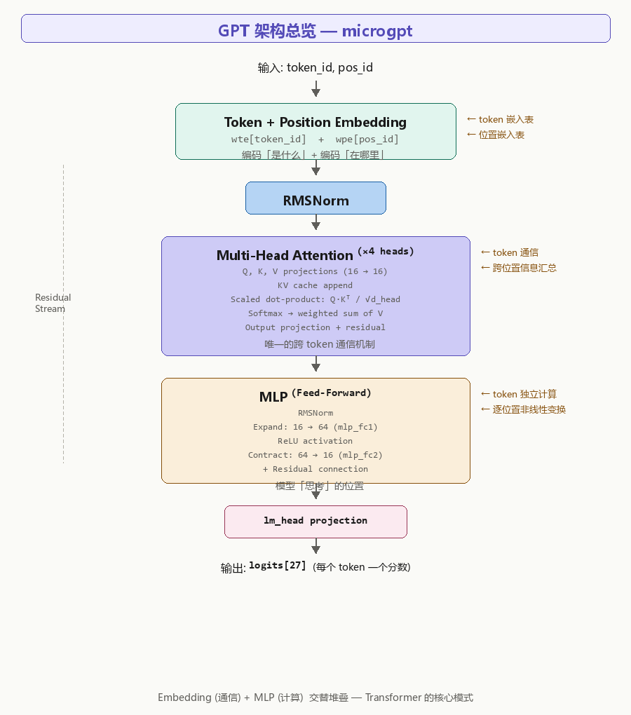
这是整份代码的心脏。gpt() 函数接收一个 token、它的位置、以及缓存的历史 K/V,输出下一个 token 的 logits(27 个分数)。
三个辅助函数
线性变换
def linear(x, w):
    return [sum(wi * xi for wi, xi in zip(wo, x)) for wo in w]
矩阵-向量乘法 w @ x。这是神经网络最基础的操作——所有”投影””变换”都是它。x 是长度为 nin 的输入向量,w 是 (nout, nin) 的权重矩阵,输出是长度为 nout 的向量。
Softmax
def softmax(logits):
    max_val = max(val.data for val in logits)
    exps = [(val - max_val).exp() for val in logits]
    total = sum(exps)
    return [e / total for e in exps]
把任意实数向量变成概率分布(非负、和为 1)。先减去最大值是为了数值稳定性——防止 exp 溢出。数学上减去常数不影响结果(分子分母同时缩放),但避免了 exp(1000) 这种灾难。
RMSNorm
def rmsnorm(x):
    ms = sum(xi * xi for xi in x) / len(x)  # 均方值
    scale = (ms + 1e-5) ** -0.5             # 缩放因子
    return [xi * scale for xi in x]         # 缩放
RMS 归一化:让向量的均方根为 1,稳定训练。它是 LayerNorm 的简化版——不做均值中心化(不减均值),只做方差缩放。1e-5 防止除零。
microgpt 用 RMSNorm 替代了 GPT-2 的 LayerNorm,这也是现代 LLM(如 LLaMA)的常见选择。
GPT 前向传播:逐段拆解
def gpt(token_id, pos_id, keys, values):
输入:
- token_id:当前 token 的 ID(整数)
- pos_id:当前位置索引(整数)
- keys/values:KV 缓存,存储之前所有位置的 K 和 V
输出:长度为 vocab_size 的 logits 列表
第一步:嵌入
tok_emb = state_dict['wte'][token_id]  # token 嵌入:查表获取"是什么"
pos_emb = state_dict['wpe'][pos_id]    # 位置嵌入:查表获取"在哪里"
x = [t + p for t, p in zip(tok_emb, pos_emb)]  # 相加融合
x = rmsnorm(x)
- wte[token_id]:从嵌入表中取出该 token 对应的 16 维向量——编码”这是什么字”
- wpe[pos_id]:从位置表中取出该位置对应的 16 维向量——编码”这是第几个字”
- 两者相加,得到同时携带”身份”和”位置”信息的表示
为什么是相加而不是拼接?相加不增加维度,更高效;而且实验证明效果足够好。
生产级 LLM 通常用 RoPE(旋转位置嵌入)替代绝对位置嵌入,因为它能更好地泛化到训练时未见过的更长序列。
第二步:多头注意力
for li in range(n_layer):
    # --- 注意力块开始 ---
    x_residual = x       # 保存残差输入
    x = rmsnorm(x)       # 归一化

    q = linear(x, state_dict[f'layer{li}.attn_wq'])  # 查询
    k = linear(x, state_dict[f'layer{li}.attn_wk'])  # 键
    v = linear(x, state_dict[f'layer{li}.attn_wv'])  # 值

    keys[li].append(k)     # 缓存当前 K
    values[li].append(v)   # 缓存当前 V
Q、K、V 的直觉:
| 向量 | 直觉 | 类比 |
| Q (Query) | “我在找什么?” | 图书馆搜索关键词 |
| K (Key) | “我包含什么?” | 书的标题/标签 |
| V (Value) | “被选中时提供什么?” | 书的内容 |
当前位置的 Q 去和所有历史位置的 K 做点积——点积越高说明越”匹配”,对应的 V 权重越大。最终输出是所有历史 V 的加权求和。
x_attn = []
for h in range(n_head):
    hs = h * head_dim
    q_h = q[hs:hs+head_dim]                          # 当前 token 在头 h 的查询
    k_h = [ki[hs:hs+head_dim] for ki in keys[li]]    # 所有历史 token 在头 h 的键
    v_h = [vi[hs:hs+head_dim] for vi in values[li]]  # 所有历史 token 在头 h 的值

    # 1) 计算注意力分数:Q 和每个 K 的点积,除以 sqrt(d) 缩放
    attn_logits = [
        sum(q_h[j] * k_h[t][j] for j in range(head_dim)) / head_dim**0.5
        for t in range(len(k_h))
    ]
    # 2) Softmax 转概率
    attn_weights = softmax(attn_logits)
    # 3) 加权求和 V
    head_out = [
        sum(attn_weights[t] * v_h[t][j] for t in range(len(v_h)))
        for j in range(head_dim)
    ]
    x_attn.extend(head_out)
为什么要除以 √d_head? 点积的方差随维度线性增长——维度越高,点积的绝对值越大,softmax 越容易饱和(变成接近 one-hot)。除以 √d 把方差拉回 1,让 softmax 有合理的梯度。
为什么要多头? 不同的头可以关注不同的模式——一个头可能学到”找元音”,另一个头可能学到”找重复字符”。4 个头各自在 4 维空间里独立做注意力,最后拼接成 16 维。
x = linear(x_attn, state_dict[f'layer{li}.attn_wo'])  # 输出投影
x = [a + b for a, b in zip(x, x_residual)]  # 残差连接
输出投影把多头拼接的结果映射回原始维度,然后加上残差(x + x_residual)。
注意力是 Transformer 中唯一的 token 间通信机制。位置 t 能”看到”过去 0..t-1 的所有 token,唯一的途径就是注意力。
第三步:MLP 块
# --- MLP 块开始 ---
x_residual = x       # 保存残差输入
x = rmsnorm(x)       # 归一化
x = linear(x, state_dict[f'layer{li}.mlp_fc1'])  # 升维:16 → 64
x = [xi.relu() for xi in x]                       # ReLU 激活
x = linear(x, state_dict[f'layer{li}.mlp_fc2'])  # 降维:64 → 16
x = [a + b for a, b in zip(x, x_residual)]        # 残差连接
MLP 是两层全连接网络:先把隐藏状态从 16 维升到 64 维(mlp_fc1),过 ReLU 激活函数,再降回 16 维(mlp_fc2)。
ReLU 做什么? relu(x) = max(0, x)——负值变 0,正值不变。这引入了非线性,让模型能学习复杂的映射关系。没有激活函数,多层线性变换等价于一层。
MLP 的角色:如果注意力是”信息汇总”(token 之间交流),那 MLP 就是”信息加工”(每个 token 独立思考)。Transformer 交替进行这两步。
microgpt 用 ReLU 替代了 GPT-2 的 GeLU——更简单,效果类似。现代 LLM 常用 SwiGLU 等门控激活。
第四步:输出
logits = linear(x, state_dict['lm_head'])  # 隐藏状态 → 词表 logits
return logits
最终隐藏状态通过 lm_head 投影到词表大小(27 维),每个维度对应一个 token 的分数。分数越高 = 模型越认为这个 token 是下一个。
关于 KV 缓存
注意 keys 和 values 参数——它们是跨 token 共享的列表。每处理一个 token,当前的 K 和 V 就被追加进去。这意味着:
- 处理第 5 个 token 时,注意力可以看到位置 0-4 的所有 K/V
- 不需要重新计算前面的 K/V——这就是 KV 缓存
生产级 LLM 在推理时大量使用 KV 缓存来加速(如 vLLM 的 PagedAttention)。microgpt 在训练时也用 KV 缓存,因为它是逐 token 处理的——缓存中的 K/V 是活跃的 Value 节点,会参与反向传播。
架构全景图
训练循环:模型如何学习
Adam 优化器
learning_rate, beta1, beta2, eps_adam = 0.01, 0.85, 0.99, 1e-8
m = [0.0] * len(params)  # 一阶矩(动量)
v = [0.0] * len(params)  # 二阶矩(梯度平方的指数移动平均)
Adam 是深度学习最常用的优化器。它结合了两个机制:
| 机制 | 变量 | 作用 |
| 动量 | m | 累积历史梯度方向,减少震荡 |
| 自适应学习率 | v | 每个参数有独立的学习率(梯度大的参数步长小) |
训练主循环
num_steps = 1000
for step in range(num_steps):
第一步:取数据并分词
doc = docs[step % len(docs)]
tokens = [BOS] + [uchars.index(ch) for ch in doc] + [BOS]
n = min(block_size, len(tokens) - 1)
每步取一个名字,两侧包裹 BOS。例如 “emma” → [BOS, e, m, m, a, BOS](token ID 序列)。n 是实际序列长度(截断到 block_size)。
第二步:前向传播 + 计算损失
keys, values = [[] for _ in range(n_layer)], [[] for _ in range(n_layer)]
losses = []
for pos_id in range(n):
    token_id, target_id = tokens[pos_id], tokens[pos_id + 1]
    logits = gpt(token_id, pos_id, keys, values)
    probs = softmax(logits)
    loss_t = -probs[target_id].log()  # 负对数似然损失
    losses.append(loss_t)
loss = (1 / n) * sum(losses)  # 序列平均损失
逐 token 前向传播:
| 位置 | 输入 token | 目标 token | 模型做什么 |
| 0 | BOS | e | 预测名字第一个字母 |
| 1 | e | m | 预测第二个字母 |
| 2 | m | m | 预测第三个字母 |
| 3 | m | a | 预测第四个字母 |
| 4 | a | BOS | 预测”名字结束” |
每个位置的损失是交叉熵(负对数似然):
- 如果模型给正确 token 的概率是0 → 损失 = 0(完美)
- 如果模型给正确 token 的概率接近 0 → 损失 → +∞(严重错误)
所有位置的损失取平均,得到这个文档的总损失。
第三步:反向传播
loss.backward()
一行代码,走完整个计算图的反向传播。之后每个参数的 .grad 告诉我们”往哪个方向调、调多少能降低损失”。
第四步:参数更新
lr_t = learning_rate * (1 - step / num_steps)  # 线性学习率衰减
for i, p in enumerate(params):
    # 更新一阶矩(动量)
    m[i] = beta1 * m[i] + (1 - beta1) * p.grad
    # 更新二阶矩(梯度平方的移动平均)
    v[i] = beta2 * v[i] + (1 - beta2) * p.grad ** 2
    # 偏差修正(因为 m、v 从 0 初始化,前期会偏小)
    m_hat = m[i] / (1 - beta1 ** (step + 1))
    v_hat = v[i] / (1 - beta2 ** (step + 1))
    # 参数更新
    p.data -= lr_t * m_hat / (v_hat ** 0.5 + eps_adam)
    p.grad = 0  # 梯度清零,为下一步做准备
偏差修正为什么需要? m 和 v 从 0 初始化,前几步的估计严重偏低。m_hat = m / (1 – β₁ᵗ) 把初始偏差除掉——当 t 很大时 β₁ᵗ → 0,修正因子趋近 1,不再有影响。
学习率衰减为什么需要? 训练初期用大学习率快速接近最优点,后期用小学习率精调,避免在最优点附近震荡。
训练过程
num docs: 32033
vocab size: 27
num params: 4192
step    1 / 1000 | loss 3.3660
step    2 / 1000 | loss 3.4243
step    5 / 1000 | loss 3.2209
step   10 / 1000 | loss 3.2229
step   50 / 1000 | loss 2.8123
step  100 / 1000 | loss 2.6451
step  500 / 1000 | loss 2.4102
step 1000 / 1000 | loss 2.3705
- 初始损失约 3 = −log(1/27) ≈ 3.3,即随机猜测
- 最终损失约 37,模型明显学到了人名的统计模式
推理:模型如何生成新内容
temperature = 0.5
print("\n--- inference (new, hallucinated names) ---")
for sample_idx in range(20):
    keys, values = [[] for _ in range(n_layer)], [[] for _ in range(n_layer)]
    token_id = BOS           # 从 BOS 开始:"开始一个新名字"
    sample = []
    for pos_id in range(block_size):
        logits = gpt(token_id, pos_id, keys, values)
        probs = softmax([l / temperature for l in logits])
        # 按概率分布随机采样
        token_id = random.choices(
            range(vocab_size),
            weights=[p.data for p in probs]
        )[0]
        if token_id == BOS:  # 模型说"我说完了"
            break
        sample.append(uchars[token_id])
    print(f"sample {sample_idx+1:2d}: {''.join(sample)}")
推理是训练的”镜像”:
- 从 BOS 开始
- 模型输出 27 个 logits → softmax 转概率
- 按概率随机采样一个 token(不是取概率最大的)
- 该 token 作为下一输入,重复
- 直到模型输出 BOS(”说完了”)或达到最大长度
Temperature 参数
在 softmax 之前把 logits 除以 temperature,控制输出的”创造性”:
| Temperature | 行为 | 类比 |
| → 0 | 几乎取概率最大的 token(贪婪解码) | 最保守,总选”最安全”的 |
| 0.5 | 锐化分布,偏向高概率 token | 适度创新 |
| 1.0 | 原始分布 | 正常采样 |
| > 1.0 | 平坦化分布,更随机 | 更多样,但可能不连贯 |
生成结果
sample  1: kamon
sample  2: ann
sample  3: karai
sample  4: jaire
sample  5: vialan
sample  6: karia
sample  7: yeran
sample  8: anna
sample  9: areli
sample 10: kaina
这些名字在训练数据中不存在——模型”幻觉”出了它们。但它们”看起来像名字”,因为模型学到了人名的统计模式(辅音开头、合理的元音辅音交替等)。
ChatGPT “幻觉”出错误信息的本质与此完全相同——模型从概率分布中采样,它没有真伪概念,只知道哪些序列在训练数据中统计上合理。
从 microgpt 到 ChatGPT:差距与桥梁
理解了 microgpt,你就理解了 GPT 的算法本质。那 ChatGPT 多了什么?
规模与工程
| 维度 | microgpt | ChatGPT |
| 参数量 | 4,192 | ~1.8 万亿 |
| 训练数据 | 32,000 个名字 | 数万亿 token 互联网文本 |
| 训练硬件 | 一台 MacBook | 数千 GPU × 数月 |
| 推理速度 | 每秒约 1 个 token | 每秒数十到上百 token |
| 数学本质 | 完全相同 | 完全相同 |
架构增强
microgpt 已经包含了 Transformer 的核心结构(注意力 + MLP + 残差 + 归一化)。现代 LLM 在此基础上增加:
- RoPE(旋转位置嵌入):替代绝对位置嵌入,更好泛化到长序列
- GQA(分组查询注意力):多个 Q 共享一组 K/V,减少 KV 缓存内存
- SwiGLU(门控激活):替代 ReLU,效果更好
- MoE(混合专家):每层只激活部分参数,用更多总参数但不增加计算量
但核心结构不变:残差流上交替的注意力通信与 MLP 计算。
后训练:从文档补全器到聊天机器人
预训练模型(包括 microgpt)只是一个文档补全器——给定前文,续写后文。它不会”对话”。ChatGPT 多了两步后训练:
- SFT(监督微调):把训练数据从”名字”换成”人写的高质量对话”,用完全相同的训练算法。模型学会”对话格式”。
- RL(强化学习):模型生成回复 → 评分(人类反馈 / 评判模型 / 规则)→ 从正负反馈中学习。此时”文档”由模型自己生成的 token 组成。
系统提示、你的消息、ChatGPT 的回复——都只是序列中的 token。模型在逐 token 补全文档,与 microgpt 补全名字在算法上完全相同。
推理工程
服务数百万用户需要巨大的工程栈:
- 批量请求:多个用户的请求合并处理
- KV 缓存管理:vLLM 的 PagedAttention 等
- 推测解码:小模型快速草拟,大模型验证
- 量化:int8/int4 降低显存和加速
- 多 GPU 分布式:模型并行、流水线并行
但核心仍然是:预测序列中的下一个 token。
渐进式学习路径
Karpathy 的教学设计是渐进式的——microgpt 是终点,但沿途有 5 个逐步演化的版本:
| 文件 | 新增内容 | 核心概念 |
| train0.py | 二元组计数表 | 无神经网络,纯统计 |
| train1.py | MLP + 手动梯度 | 神经网络入门,数值/解析梯度 |
| train2.py | 自动微分(Value 类) | 告别手动求导 |
| train3.py | 位置嵌入 + 单头注意力 + 残差 | Transformer 雏形 |
| train4.py | 多头注意力 + 层循环 | 完整 GPT 架构 |
| train5.py | Adam 优化器 | 即最终的 microgpt.py |
建议按此顺序学习,每一步只引入一个新概念,确保完全理解后再进入下一步。
动手实验建议
快速运行
只需 Python 3,无需 pip install 任何东西。MacBook 上约 1 分钟跑完。
有趣的修改
- 更换数据集:把 txt 换成城市名、宝可梦名、英文单词或短诗——模型会学会生成这些。其余代码无需修改。
- 增大模型:调大 n_embd、n_layer、n_head——但纯 Python 会更慢。
- 增加训练步数:把 num_steps 从 1000 改到 5000——损失会更低,生成质量更好。
- 调整 Temperature:从1 到 2.0,观察生成名字的多样性变化。
- 观察注意力权重:在 gpt() 函数中打印 attn_weights,看模型在不同位置关注哪些 token。
总结:一份代码,一个宇宙
microgpt 用 200 行纯 Python 实现了一个完整的 GPT。没有 PyTorch 的黑盒、没有 CUDA 的迷雾——每一步计算都透明可见。
完整代码:
""" The most atomic way to train and run inference for a GPT in pure, dependency-free Python. This file is the complete algorithm. Everything else is just efficiency. @karpathy """
import os       # os.path.exists
import math     # math.log, math.exp
import random   # random.seed, random.choices, random.gauss, random.shuffle

random.seed(42)  # Let there be order among chaos

# Let there be a Dataset `docs`: list[str] of documents (e.g. a list of names)
if not os.path.exists('input.txt'):
    import urllib.request
    names_url = 'https://raw.githubusercontent.com/karpathy/makemore/988aa59/names.txt'
    urllib.request.urlretrieve(names_url, 'input.txt')
docs = [line.strip() for line in open('input.txt') if line.strip()]
random.shuffle(docs)
print(f"num docs: {len(docs)}")

# Let there be a Tokenizer to translate strings to sequences of integers ("tokens") and back
uchars = sorted(set(''.join(docs)))  # unique characters in the dataset become token ids 0..n-1
BOS = len(uchars)  # token id for a special Beginning of Sequence (BOS) token
vocab_size = len(uchars) + 1  # total number of unique tokens, +1 is for BOS
print(f"vocab size: {vocab_size}")

# Let there be Autograd to recursively apply the chain rule through a computation graph
class Value:
    __slots__ = ('data', 'grad', '_children', '_local_grads')  # Python optimization for memory usage

    def __init__(self, data, children=(), local_grads=()):
        self.data = data  # scalar value of this node calculated during forward pass
        self.grad = 0     # derivative of the loss w.r.t. this node, calculated in backward pass
        self._children = children  # children of this node in the computation graph
        self._local_grads = local_grads  # local derivative of this node w.r.t. its children

    def __add__(self, other):
        other = other if isinstance(other, Value) else Value(other)
        return Value(self.data + other.data, (self, other), (1, 1))

    def __mul__(self, other):
        other = other if isinstance(other, Value) else Value(other)
        return Value(self.data * other.data, (self, other), (other.data, self.data))

    def __pow__(self, other):
        return Value(self.data**other, (self,), (other * self.data**(other-1),))

    def log(self):
        return Value(math.log(self.data), (self,), (1/self.data,))

    def exp(self):
        return Value(math.exp(self.data), (self,), (math.exp(self.data),))

    def relu(self):
        return Value(max(0, self.data), (self,), (float(self.data > 0),))

    def __neg__(self):
        return self * -1

    def __radd__(self, other):
        return self + other

    def __sub__(self, other):
        return self + (-other)

    def __rsub__(self, other):
        return other + (-self)

    def __rmul__(self, other):
        return self * other

    def __truediv__(self, other):
        return self * other**-1

    def __rtruediv__(self, other):
        return other * self**-1

    def backward(self):
        topo = []
        visited = set()

        def build_topo(v):
            if v not in visited:
                visited.add(v)
                for child in v._children:
                    build_topo(child)
                topo.append(v)
        build_topo(self)
        self.grad = 1
        for v in reversed(topo):
            for child, local_grad in zip(v._children, v._local_grads):
                child.grad += local_grad * v.grad

# Initialize the parameters, to store the knowledge of the model
n_layer = 1       # depth of the transformer neural network (number of layers)
n_embd = 16       # width of the network (embedding dimension)
block_size = 16   # maximum context length of the attention window (note: the longest name is 15 characters)
n_head = 4        # number of attention heads
head_dim = n_embd // n_head  # derived dimension of each head

matrix = lambda nout, nin, std=0.08: [[Value(random.gauss(0, std)) for _ in range(nin)] for _ in range(nout)]
state_dict = {'wte': matrix(vocab_size, n_embd), 'wpe': matrix(block_size, n_embd), 'lm_head': matrix(vocab_size, n_embd)}
for i in range(n_layer):
    state_dict[f'layer{i}.attn_wq'] = matrix(n_embd, n_embd)
    state_dict[f'layer{i}.attn_wk'] = matrix(n_embd, n_embd)
    state_dict[f'layer{i}.attn_wv'] = matrix(n_embd, n_embd)
    state_dict[f'layer{i}.attn_wo'] = matrix(n_embd, n_embd)
    state_dict[f'layer{i}.mlp_fc1'] = matrix(4 * n_embd, n_embd)
    state_dict[f'layer{i}.mlp_fc2'] = matrix(n_embd, 4 * n_embd)
params = [p for mat in state_dict.values() for row in mat for p in row]  # flatten params into a single list[Value]
print(f"num params: {len(params)}")

# Define the model architecture: a function mapping tokens and parameters to logits over what comes next
# Follow GPT-2, blessed among the GPTs, with minor differences: layernorm -> rmsnorm, no biases, GeLU -> ReLU
def linear(x, w):
    return [sum(wi * xi for wi, xi in zip(wo, x)) for wo in w]

def softmax(logits):
    max_val = max(val.data for val in logits)
    exps = [(val - max_val).exp() for val in logits]
    total = sum(exps)
    return [e / total for e in exps]

def rmsnorm(x):
    ms = sum(xi * xi for xi in x) / len(x)
    scale = (ms + 1e-5) ** -0.5
    return [xi * scale for xi in x]

def gpt(token_id, pos_id, keys, values):
    tok_emb = state_dict['wte'][token_id]  # token embedding
    pos_emb = state_dict['wpe'][pos_id]    # position embedding
    x = [t + p for t, p in zip(tok_emb, pos_emb)]  # joint token and position embedding
    x = rmsnorm(x)  # note: not redundant due to backward pass via the residual connection

    for li in range(n_layer):
        # 1) Multi-head Attention block
        x_residual = x
        x = rmsnorm(x)
        q = linear(x, state_dict[f'layer{li}.attn_wq'])
        k = linear(x, state_dict[f'layer{li}.attn_wk'])
        v = linear(x, state_dict[f'layer{li}.attn_wv'])
        keys[li].append(k)
        values[li].append(v)
        x_attn = []
        for h in range(n_head):
            hs = h * head_dim
            q_h = q[hs:hs+head_dim]
            k_h = [ki[hs:hs+head_dim] for ki in keys[li]]
            v_h = [vi[hs:hs+head_dim] for vi in values[li]]
            attn_logits = [sum(q_h[j] * k_h[t][j] for j in range(head_dim)) / head_dim**0.5 for t in range(len(k_h))]
            attn_weights = softmax(attn_logits)
            head_out = [sum(attn_weights[t] * v_h[t][j] for t in range(len(v_h))) for j in range(head_dim)]
            x_attn.extend(head_out)
        x = linear(x_attn, state_dict[f'layer{li}.attn_wo'])
        x = [a + b for a, b in zip(x, x_residual)]

        # 2) MLP block
        x_residual = x
        x = rmsnorm(x)
        x = linear(x, state_dict[f'layer{li}.mlp_fc1'])
        x = [xi.relu() for xi in x]
        x = linear(x, state_dict[f'layer{li}.mlp_fc2'])
        x = [a + b for a, b in zip(x, x_residual)]

    logits = linear(x, state_dict['lm_head'])
    return logits

# Let there be Adam, the blessed optimizer and its buffers
learning_rate, beta1, beta2, eps_adam = 0.01, 0.85, 0.99, 1e-8
m = [0.0] * len(params)  # first moment buffer
v = [0.0] * len(params)  # second moment buffer

# Repeat in sequence
num_steps = 1000  # number of training steps
for step in range(num_steps):
    # Take single document, tokenize it, surround it with BOS special token on both sides
    doc = docs[step % len(docs)]
    tokens = [BOS] + [uchars.index(ch) for ch in doc] + [BOS]
    n = min(block_size, len(tokens) - 1)

    # Forward the token sequence through the model, building up the computation graph all the way to the loss
    keys, values = [[] for _ in range(n_layer)], [[] for _ in range(n_layer)]
    losses = []
    for pos_id in range(n):
        token_id, target_id = tokens[pos_id], tokens[pos_id + 1]
        logits = gpt(token_id, pos_id, keys, values)
        probs = softmax(logits)
        loss_t = -probs[target_id].log()
        losses.append(loss_t)
    loss = (1 / n) * sum(losses)  # final average loss over the document sequence. May yours be low.

    # Backward the loss, calculating the gradients with respect to all model parameters
    loss.backward()

    # Adam optimizer update: update the model parameters based on the corresponding gradients
    lr_t = learning_rate * (1 - step / num_steps)  # linear learning rate decay
    for i, p in enumerate(params):
        m[i] = beta1 * m[i] + (1 - beta1) * p.grad
        v[i] = beta2 * v[i] + (1 - beta2) * p.grad ** 2
        m_hat = m[i] / (1 - beta1 ** (step + 1))
        v_hat = v[i] / (1 - beta2 ** (step + 1))
        p.data -= lr_t * m_hat / (v_hat ** 0.5 + eps_adam)
        p.grad = 0
    print(f"step {step+1:4d} / {num_steps:4d} | loss {loss.data:.4f}", end='\r')

# Inference: may the model babble back to us
temperature = 0.5  # in (0, 1], control the "creativity" of generated text, low to high
print("\n--- inference (new, hallucinated names) ---")
for sample_idx in range(20):
    keys, values = [[] for _ in range(n_layer)], [[] for _ in range(n_layer)]
    token_id = BOS
    sample = []
    for pos_id in range(block_size):
        logits = gpt(token_id, pos_id, keys, values)
        probs = softmax([l / temperature for l in logits])
        token_id = random.choices(range(vocab_size), weights=[p.data for p in probs])[0]
        if token_id == BOS:
            break
        sample.append(uchars[token_id])
    print(f"sample {sample_idx+1:2d}: {''.join(sample)}")
回顾全文的核心洞察:
- 数据是模型的世界:模型只”知道”训练数据中的统计模式
- 分词是文本到数字的桥梁:字符、子词、token——本质都是整数
- 自动微分是学习的引擎:链式法则 + 拓扑排序 = 反向传播
- Transformer = 注意力(通信)+ MLP(计算):交替堆叠,残差连接
- 训练 = 前向 → 损失 → 反向 → 更新:循环重复,损失下降
- 推理 = 预测下一 token → 采样 → 重复:就这么简单
- ChatGPT = microgpt + 规模 + 后训练:算法本质完全相同
“如果你理解了 microgpt,你就理解了 LLM 算法的本质。其余的一切都只是效率问题。”
这不是终点,而是起点。当你理解了这 200 行代码,再去看 PyTorch 文档、去看 LLaMA 论文、去看 vLLM 源码——你会发现它们都是在这份骨架上添砖加瓦。算法的骨架,就在这里。